The first XAI library grounded in Riemannian information geometry
Prof. Dr. Utku Kose
Suleyman Demirel University, Turkey · University of North Dakota, USA · VelTech University, India · Universidad Panamericana, Mexico
GEMEX explains any machine learning model — tabular data, time series, or images — by measuring the true curved geometry of its prediction surface, rather than approximating it as flat.
pip install gemexfrom gemex import Explainer, GemexConfig
cfg = GemexConfig(n_geodesic_steps=20, n_reference_samples=60,
interaction_order=2)
exp = Explainer(model, data_type='tabular',
feature_names=feature_names,
class_names=['No','Yes'], config=cfg)
result = exp.explain(x_instance, X_reference=X_train)
print(result.summary())
print(result.top_features(5))
print(result.top_interactions(3))
print(f"Ricci: {result.manifold_curvature:.4f} FIM: {result.fim_quality}")
# All 13 visualisation types — dark and light themes
result.plot("gsf_bar", theme="dark")
result.plot("force", theme="dark")
result.plot("waterfall", theme="dark")
result.plot("heatmap", theme="dark")
result.plot("beeswarm", theme="dark", batch_results=batch)
result.plot("network", theme="dark")
result.plot("curvature", theme="dark")
result.plot("attention_heatmap", theme="dark")
result.plot("attention_dwell", theme="dark")
result.plot("attention_vs_effect", theme="dark")
result.plot("bias", theme="dark")
result.plot("image_trio", theme="dark") # image data only
result.plot("triplet_hypergraph", theme="dark") # interaction_order=3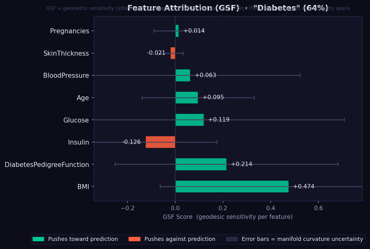
What it shows: Each bar is a signed Geodesic Sensitivity Field (GSF) score — how strongly each feature pushes the model's prediction toward or against the predicted class, measured by integrating directional sensitivity along the curved geodesic path on the statistical manifold.
How to read it:
- 🟢 Green bar → feature supports the predicted class. Longer = stronger.
- 🔴 Red/orange bar → feature opposes the predicted class.
- Error bars → curvature-weighted geometric uncertainty. Width reflects how much the manifold curves in that feature's direction. Wide bars mean the model's surface is geometrically complex near this feature — a confidence indicator exclusive to GEMEX (unavailable in SHAP or LIME).
- Features are sorted by absolute importance (most important at bottom).
- Unlike SHAP values, GSF scores are reparametrisation-invariant: rescaling a feature (e.g. cm → metres) does not change its attribution.
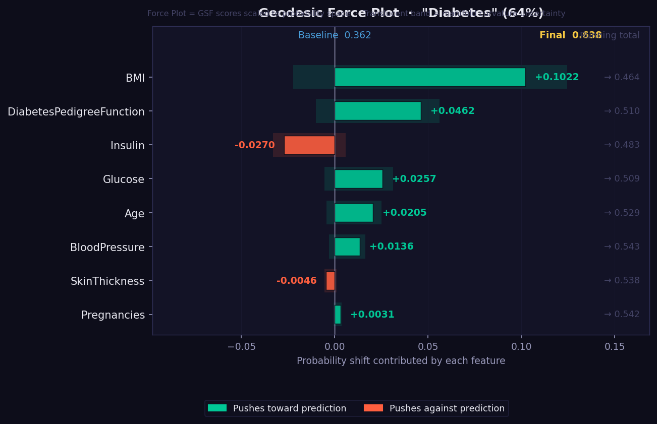
What it shows: A waterfall-style push/pull visualisation showing how the prediction probability is built up from a baseline value through the contributions of each feature.
How to read it:
- The plot reads left-to-right from baseline probability to final prediction.
- 🟢 Green segments push the probability upward (toward the predicted class).
- 🔴 Red segments pull it downward.
- Feature order follows actual attribution magnitude — the largest movers appear first.
- The final bar position shows the predicted probability.
- Useful for explaining a single prediction to a non-technical stakeholder: "your prediction starts at the average of 0.5 and these factors moved it to 0.73."
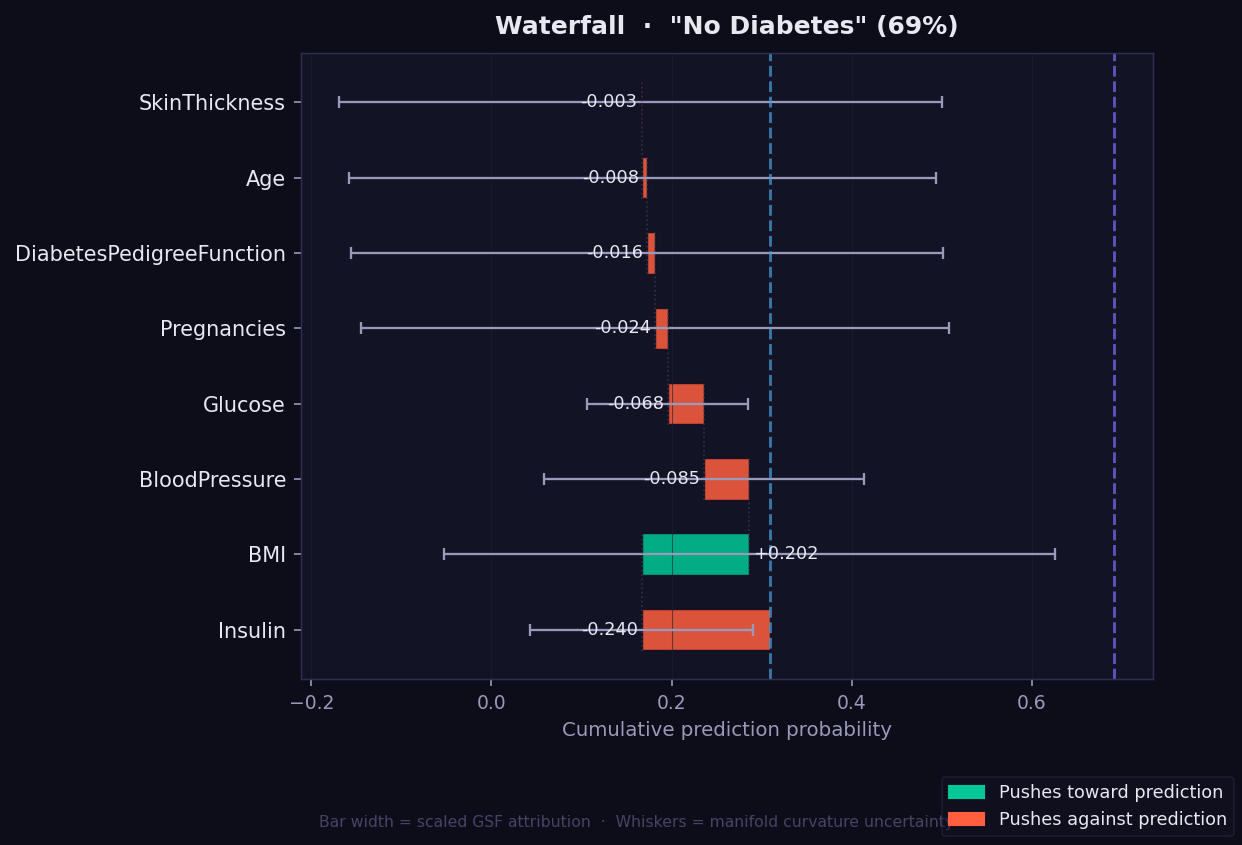
What it shows: A step-by-step view of how each feature moves the prediction from the baseline probability to the final value, based on its GSF attribution along the geodesic path. Each bar starts where the previous one ended, making the accumulation explicit and traceable.
How to read it:
- Read left to right: the dotted left line is the baseline, the right line is the final prediction.
- 🟢 Green bar → feature pushes prediction toward the predicted class.
- 🔴 Red/orange bar → feature pulls prediction away.
- Whisker on each bar → curvature-weighted geometric uncertainty, exclusive to GEMEX.
- Number labels → original GSF score for that feature (not rescaled).
- Unlike the Force plot which shows a push-pull summary, the Waterfall shows exact numerical steps — useful when you need to communicate the precise contribution of each feature to a clinical or technical audience.
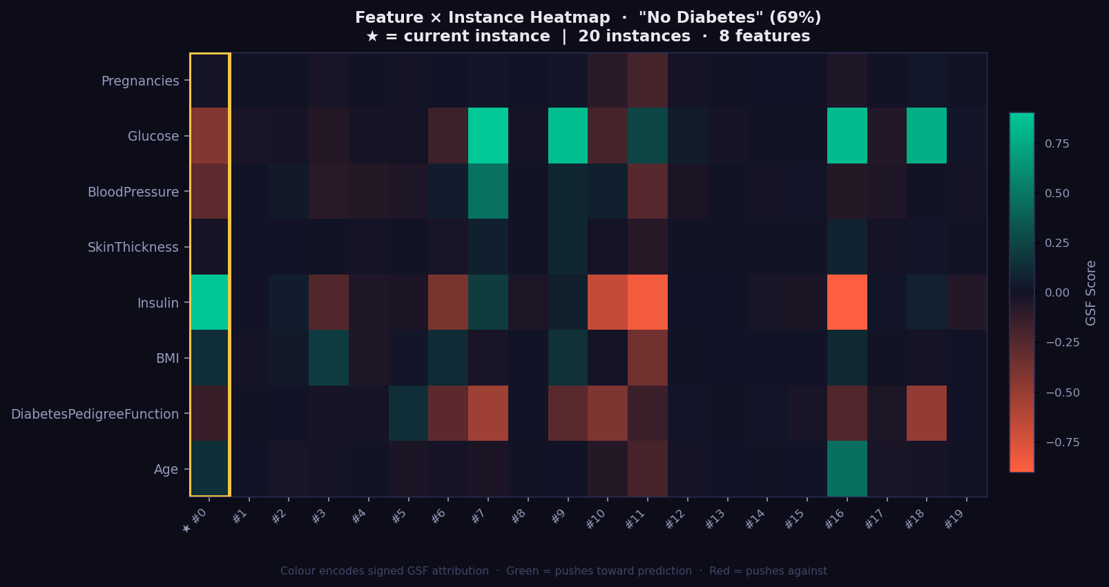
What it shows: A 2D grid of GSF attributions across a batch of instances — rows are features, columns are instances. This gives you a population-level view of which features drive predictions consistently and which vary by individual.
How to read it:
- 🟢 Green cell → feature strongly supports the predicted class for that instance.
- 🔴 Red cell → feature works against the prediction.
- Dark cell → near-zero attribution; feature irrelevant for that instance.
- Gold-bordered column → the currently explained instance (highlighted for reference).
- Consistent green/red column → the model relies on this feature across all instances.
- Highly variable column → attribution is instance-specific; investigate individually.
- Run
exp.explain_batch(X_test[:20])first, then passbatch_results=batchas argument. - Most valuable with 10–50 instances to reveal systematic patterns and outlier explanations.
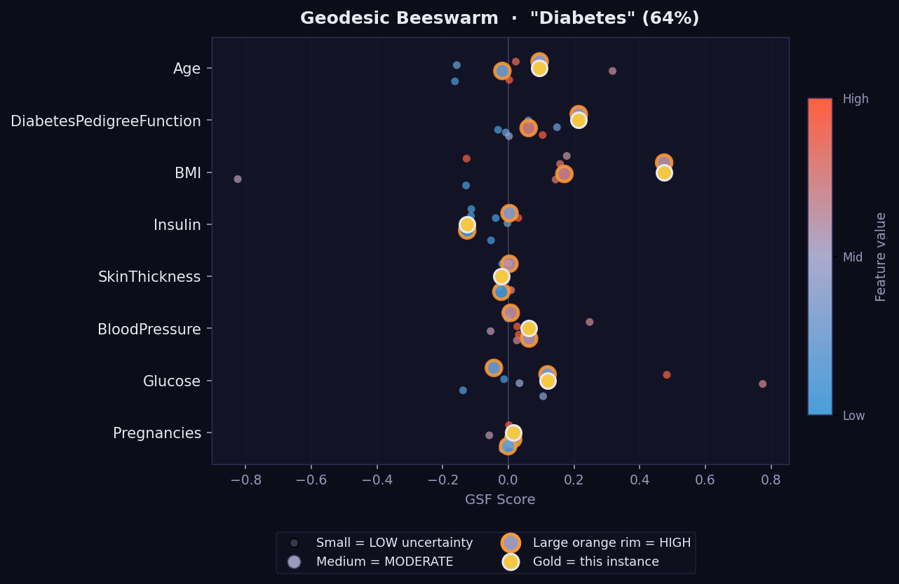
What it shows: A global view of attribution distributions across a batch of instances — the GEMEX equivalent of SHAP's beeswarm summary plot.
How to read it:
- Each dot is one instance. Dots are spread vertically to avoid overlap.
- Horizontal position → GSF attribution value (positive right, negative left).
- Dot colour → feature value (warm = high, cool = low) using the original scale.
- Wide horizontal spread = feature has variable importance across instances.
- Narrow cluster near zero = feature rarely matters regardless of its value.
- Requires
batch_results=batchargument. Runexp.explain_batch(X_test[:50])first.
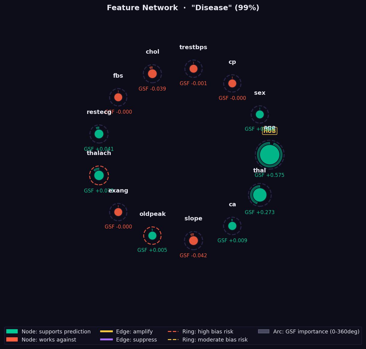
What it shows: A graph of pairwise feature interactions measured via Parallel Transport Interaction (PTI) — the holonomy angle accumulated when parallel-transporting a feature's attribution vector around a closed loop on the statistical manifold.
How to read it:
- Node size → absolute GSF importance. Larger = more important.
- 🟢 Green node → feature supports the prediction.
- 🔴 Red node → feature opposes the prediction.
- Edge thickness → strength of the nonlinear interaction. Thick = strong co-dependency that no additive method (SHAP, LIME) can capture.
- 🟡 Yellow edge → amplifying interaction (features reinforce each other).
- 🟣 Purple edge → suppressing interaction (features partially cancel).
- Dashed ring → Bias Trap risk (geodesic over-attends this feature).
- "HUB" label → high geometric interaction with many other features.
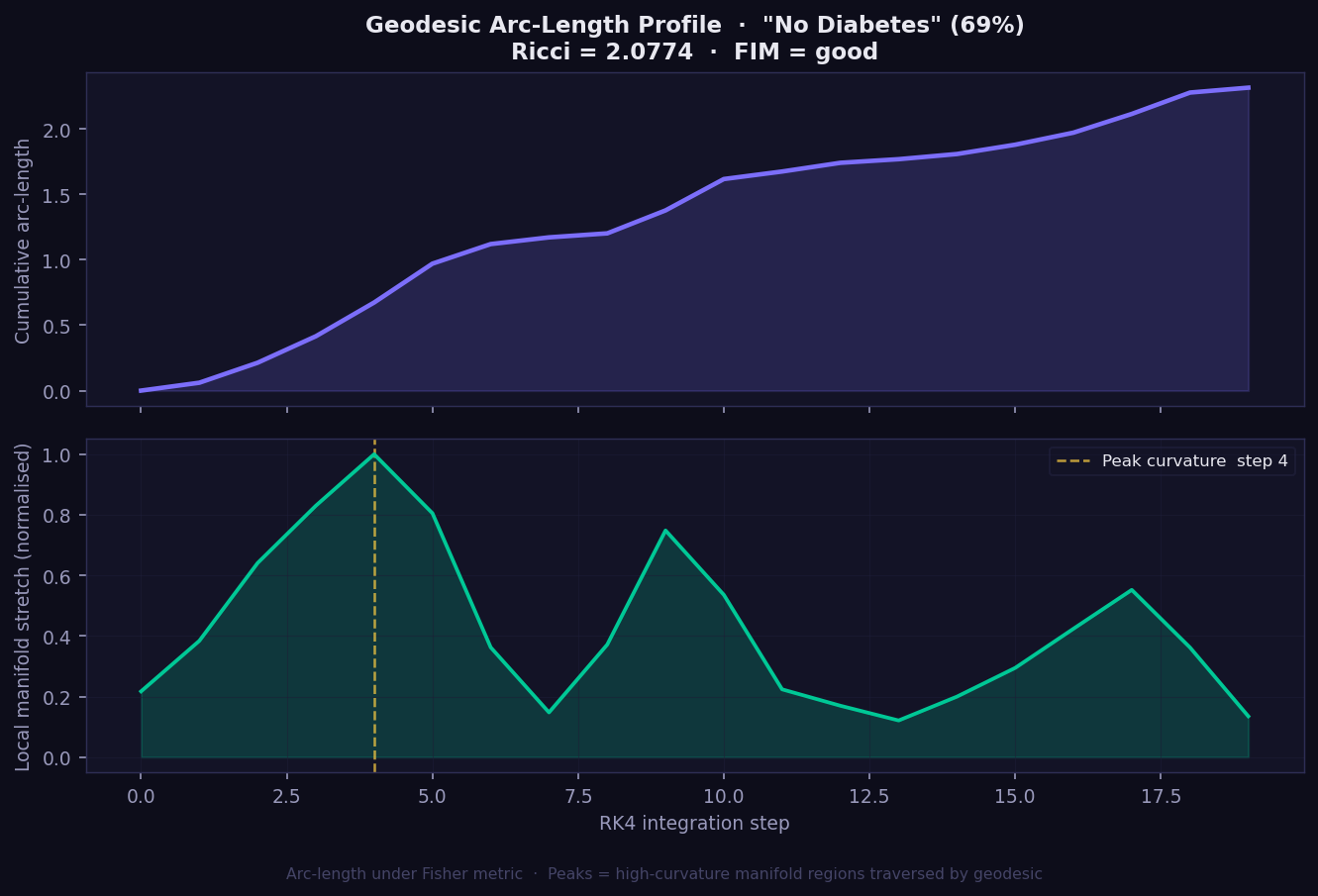
What it shows: The geometric journey the explanation takes from baseline to prediction, plotted as two panels. The top panel shows cumulative Fisher-Rao arc-length — how far the geodesic has travelled on the statistical manifold at each integration step. The bottom panel shows local manifold stretch — how much the surface bends at each step along the path.
How to read it:
- Top panel (cumulative arc-length): A steadily rising curve means the manifold is smooth; steep jumps indicate high-curvature zones the geodesic crosses. SHAP and Integrated Gradients assume this would be a straight line — GEMEX shows you where that assumption breaks down.
- Bottom panel (local stretch): Peaks mark where the model's decision surface curves most sharply. The gold dashed line marks the single step of peak curvature.
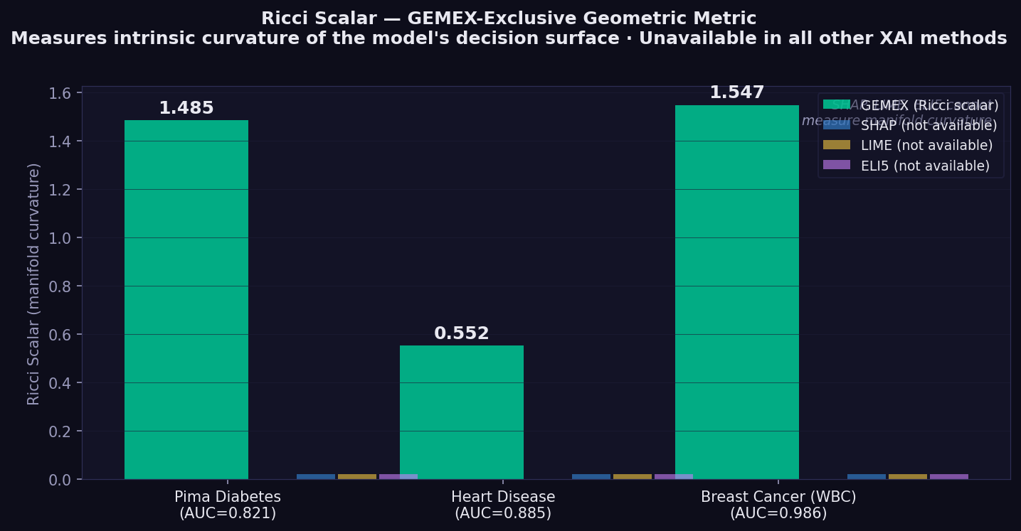
- Ricci scalar in title: The single-number summary of overall manifold curvature for this instance. Higher = prediction in a more geometrically complex region.
- FIM = good/marginal/poor: Quality indicator of the Fisher metric estimation. Only interpret Ricci confidently when FIM = good.
- No equivalent plot exists in SHAP, LIME, or GradCAM. This view of the model's internal geometry is exclusive to GEMEX.
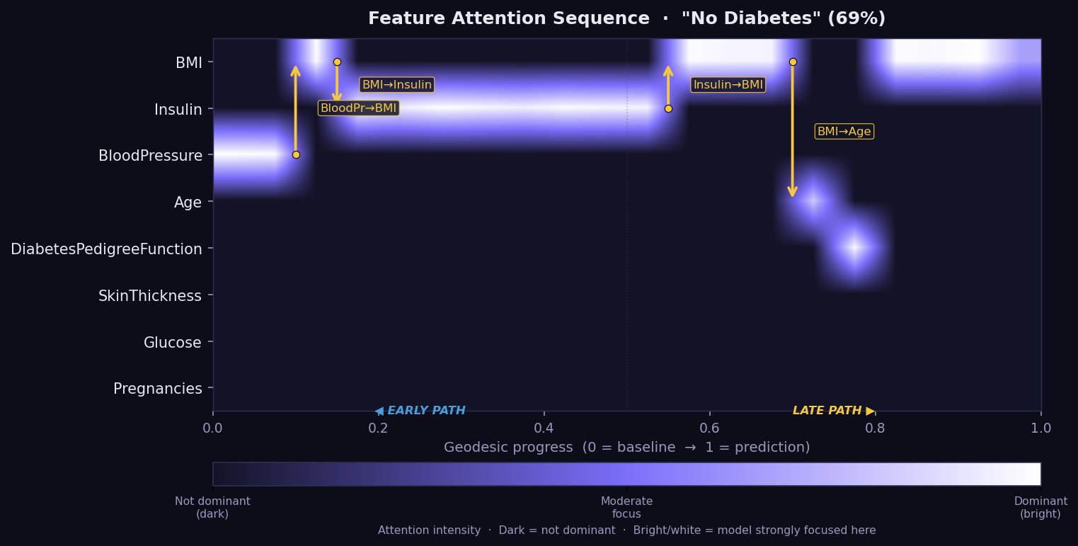
What it shows: The Feature Attention Sequence (FAS) — a temporal map of which features the geodesic path moves through, and for how long, on its journey from the baseline to the explained instance. Think of it as a recording of the model's geometric reasoning process, step by step. No other XAI method captures this temporal dimension of explanation.
How to read it:
- X-axis = geodesic progress from 0 (baseline) to 1 (prediction).
- Y-axis = features. Brightness = attention intensity at that step.
- Bright horizontal band → the model's geodesic spends extended time in this feature's direction — it is geometrically dominant during that phase of the path.
- Gold arrows → attention transitions: the path shifts focus from one feature to another, labelled with the direction (e.g. "BMI→Insulin").
- Early path (left) = the initial reasoning phase from baseline. Late path (right) = refinement near the final prediction.
- If a feature appears bright in the FAS but has a low GSF bar, it may be a Bias Trap candidate — the model attends to it without converting attention into final attribution. Cross-check with the Bias plot.
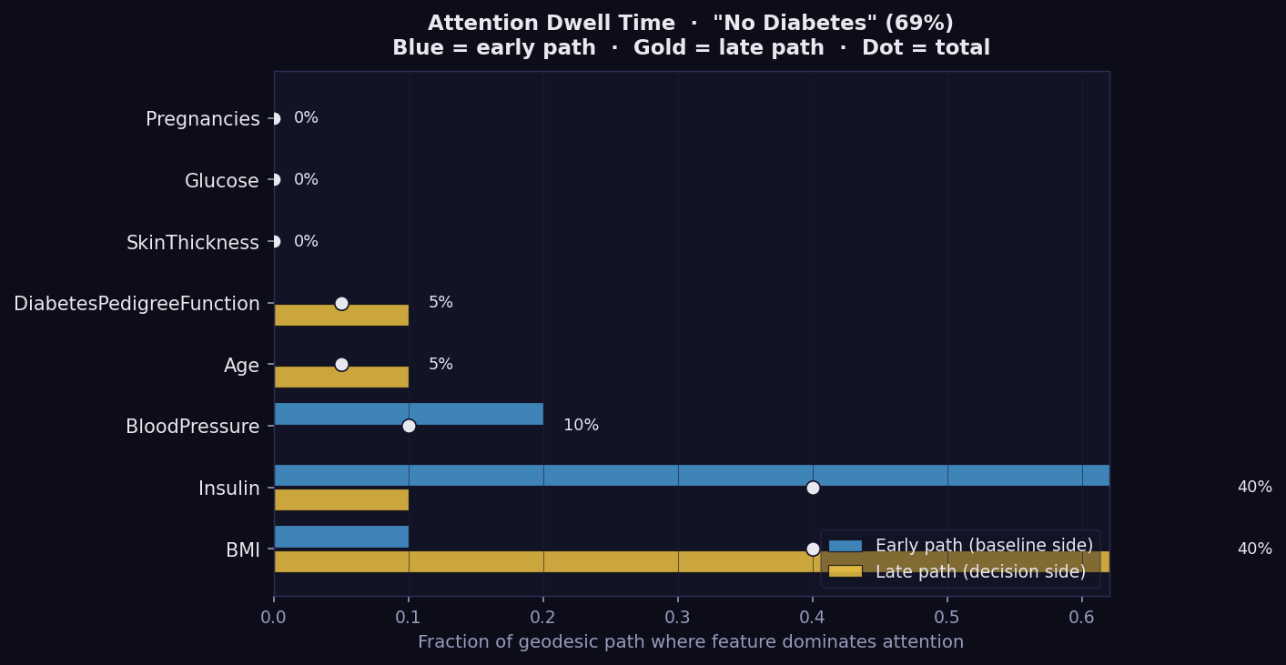
What it shows: Per-feature geodesic dwell time as a bar chart for one instance, split into early path (blue, baseline side) and late path (gold, decision side). This is the most compact way to see where the model's geometric attention is concentrated during the explanation journey.
How to read it:
- Longer bar → the geodesic spends a greater fraction of its path near this feature's axis. The model is geometrically attentive to it.
- Blue (early path) → attention concentrated near the baseline. The feature influences the reasoning from the start.
- Gold (late path) → attention concentrated near the final prediction. The feature becomes important only as the path approaches the decision boundary.
- Percentage label → total fraction of the geodesic path where this feature dominates attention.
- Features with high dwell but low GSF attribution are Bias Trap candidates — the model spends time on them without converting that attention into final output. Cross-check against the Bias plot.
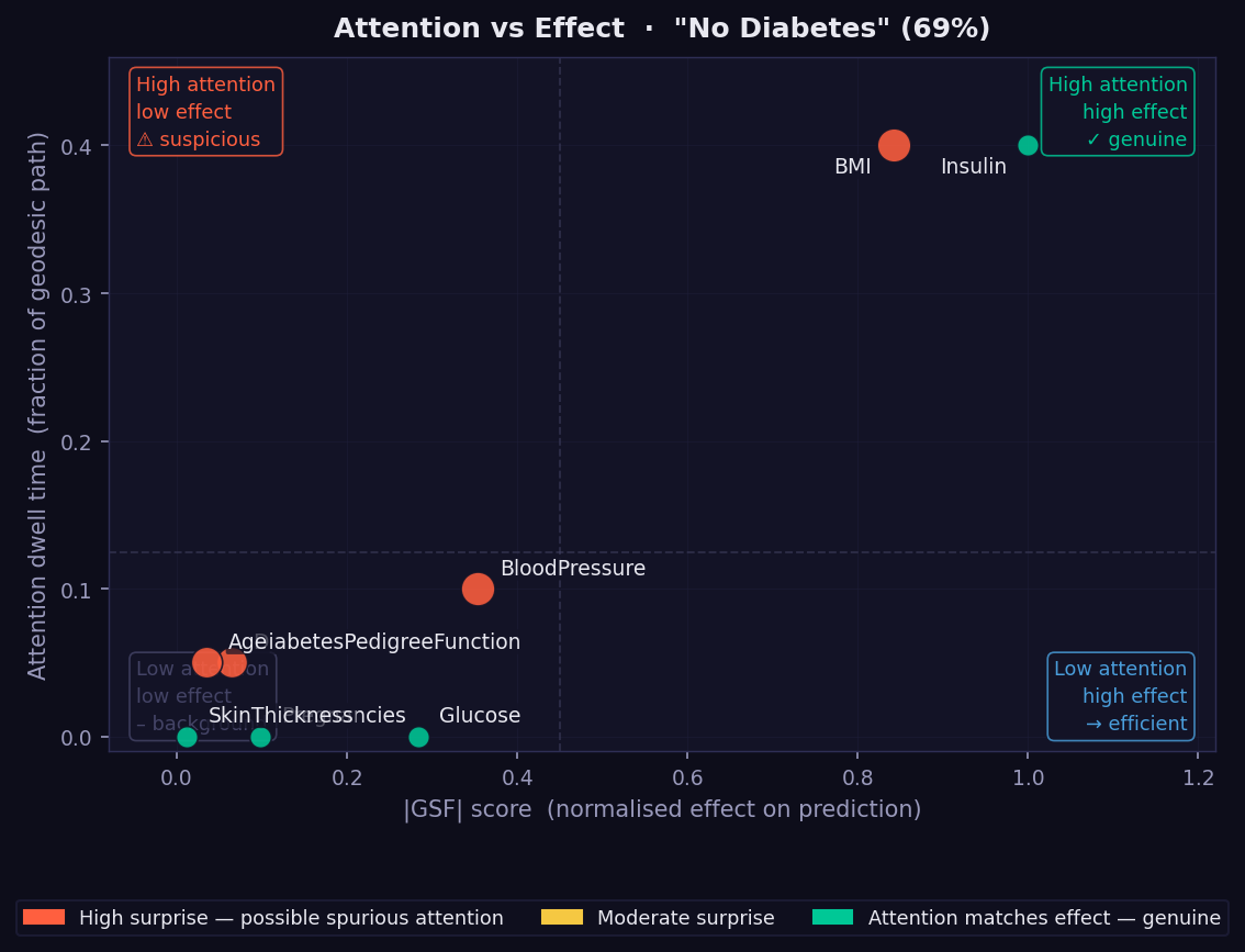
What it shows: A scatter plot placing every feature at the intersection of its geodesic dwell time (y-axis) and its absolute GSF attribution (x-axis). The four quadrants each have a distinct interpretation, labelled directly on the plot.
How to read it:
- Top-right (high attention, high effect — genuine) → the model both attends to and acts on these features. These are the most trustworthy attributions.
- Top-left (high attention, low effect — suspicious) → potential Bias Trap. The model spends geometric attention here without converting it into final output. Flag for review, especially for sensitive attributes.
- Bottom-right (low attention, high effect — efficient) → the model resolves these features quickly and sharply. Attribution is concentrated and local.
- Bottom-left (low attention, low effect — background) → features the model largely ignores for this instance.
- Dot colour → orange = high surprise (dwell and effect mismatched); green = genuine (dwell proportionate to effect).
- Dot size → relative magnitude of the mismatch.

What it shows: A diagnostic for geometric bias — features where the model spends disproportionate geodesic attention relative to the final attribution they receive. This is a GEMEX-exclusive audit tool with no equivalent in SHAP, LIME, or GradCAM. Each bar is a stacked score from three independent geometric indicators.
How to read it:
- 🔴 HAT (Holonomy Asymmetry Test) → detects confounder signals: the feature generates asymmetric curvature loops, suggesting the model responds differently depending on context rather than the feature's direct value.
- 🟡 MCA (Manifold Curvature Asymmetry) → flags over-reliance: unusually high curvature in this feature's direction without proportionate GSF attribution.
- 🟣 GDI (Geodesic Dominance Inconsistency) → identifies spurious correlation: high attention dwell combined with low final effect.
- H / M / L labels → overall risk level: High, Moderate, or Low.
- Features marked H — especially age, sex, or ethnicity — should be reviewed before deploying the model in clinical or regulatory contexts.
- A feature can be important (high GSF) and low-risk, or unimportant and high-risk. The Bias plot captures something the attribution bars cannot.
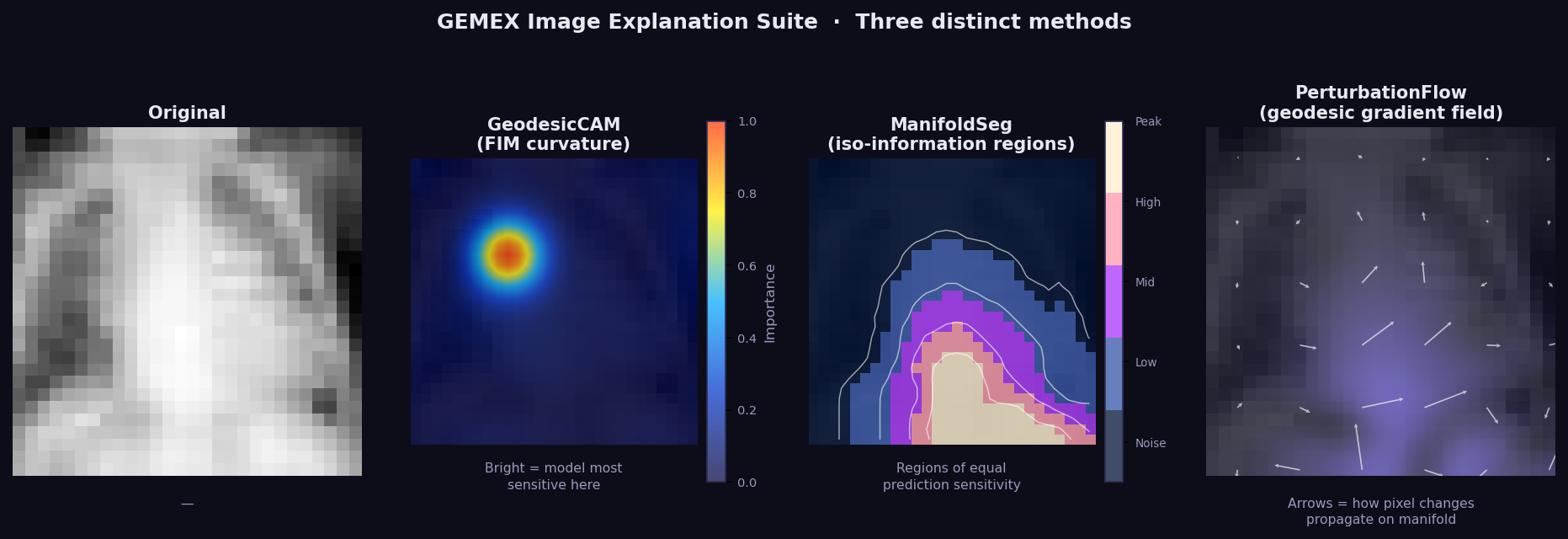
What it shows: Three-panel image explanation for data_type='image':
- Panel 1 (Original) — the input image.
- Panel 2 (GeodesicCAM) — GSF attribution upsampled to pixel space. Bright regions = model most sensitive here along the geodesic path. Model-agnostic equivalent of GradCAM — no CNN access required.
- Panel 3 (ManifoldSeg) — iso-information regions: areas where the model's prediction sensitivity is approximately equal. Similar to a level-set of the probability function on the manifold.
- Panel 4 (PerturbFlow) — geodesic gradient field: arrows show how pixel changes would propagate on the manifold surface.
How to read it: Bright GeodesicCAM regions are the most discriminative for the prediction. ManifoldSeg boundaries separate regions of qualitatively different model sensitivity. PerturbFlow arrows show the local direction of maximum prediction change.
GEMEX image_trio on PneumoniaMNIST (Pneumonia class). GeodesicCAM correctly
identifies the left upper lobe as the dominant region using only predict_proba()
— no CNN layer access required.
Requires interaction_order=3 in GemexConfig.
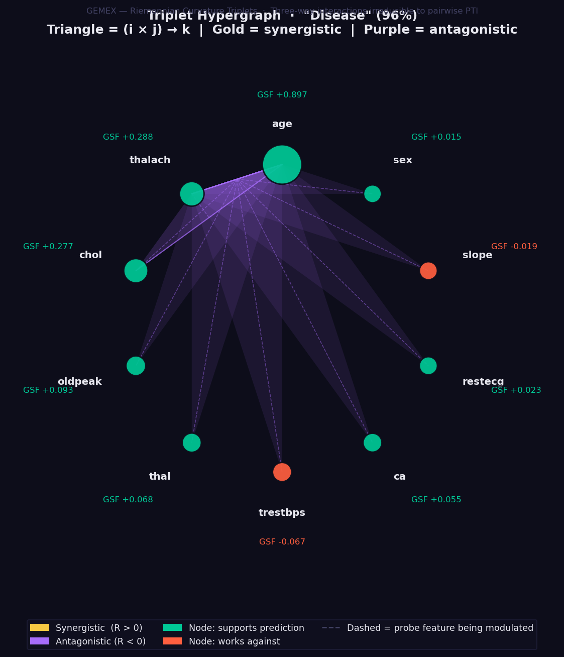
What it shows: Three-way feature interactions computed via the Riemannian Curvature Triplet (RCT) — the only XAI method in existence that quantifies how a third feature modulates the interaction between two others, derived directly from the Riemann curvature tensor of the statistical manifold.
This goes beyond pairwise interaction methods: a non-zero RCT(i, j, k) means that the relationship between features i and j changes depending on the value of feature k. No combination of SHAP interaction values, LIME coefficients, or PTI scores can capture this three-way modulation.
How to read it:
- Feature nodes sit on a circle, sized by absolute GSF attribution magnitude.
- 🟢 Green node → feature supports the prediction. 🔴 Red → works against.
- Each triangle connects three features (i × j → k):
- 🟡 Gold triangle → synergistic: together these three features reinforce each other beyond what pairwise analysis would suggest.
- 🟣 Purple triangle → antagonistic: the three-way combination partially cancels or suppresses the individual contributions.
- Triangle opacity → magnitude of the RCT value. Opaque = strong interaction.
- Dashed line → the probe feature k being modulated by the i-j pair.
- Note: set
interaction_order=3inGemexConfig. This is slower thaninteraction_order=2because C(n_features, 3) tensor entries are computed. For 13 features that is 286 triplets. Start withn_geodesic_steps=12to balance speed and quality.
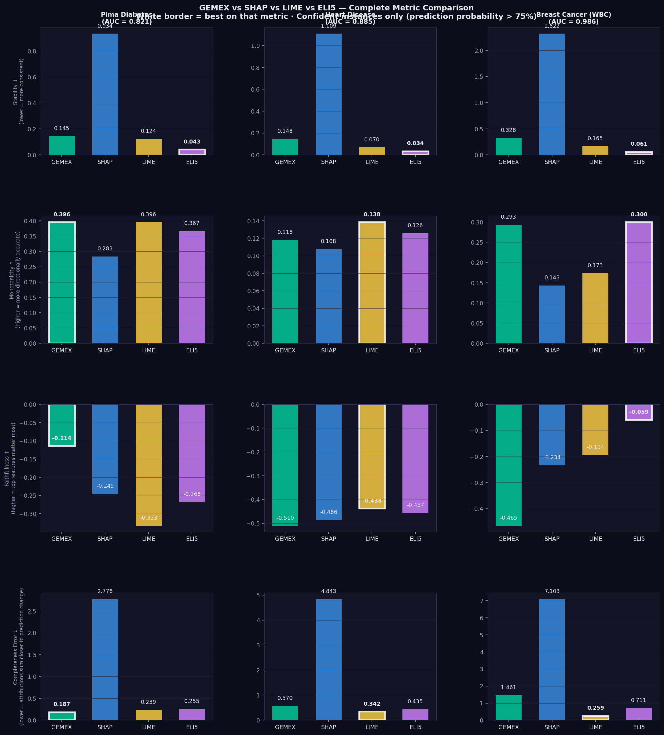
These results are to appear in a peer-reviewed study. Currently submitted to IEEE HORA 2026. Three datasets × three model families (GBM, MLP, DeepMLP) × 5 random seeds.
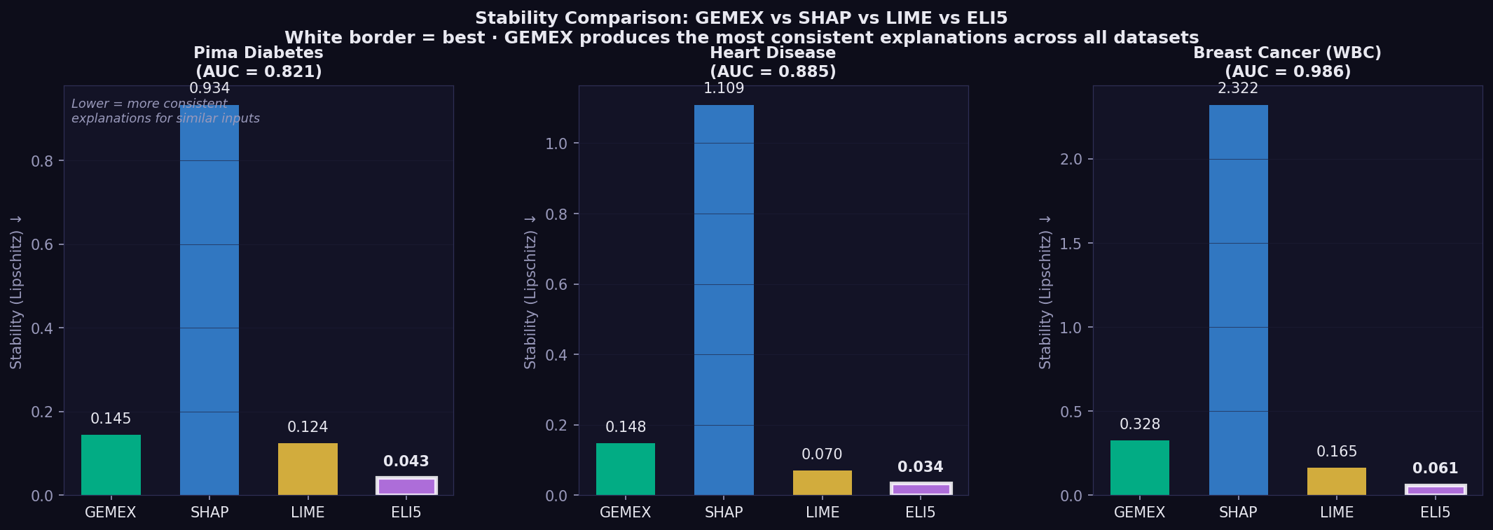
Across all three datasets and all model families, GEMEX produces the most consistent explanations for similar inputs (Lipschitz stability metric, lower is better):
| Dataset | GEMEX | SHAP | Ratio |
|---|---|---|---|
| Pima Diabetes (GBM) | 0.145 | 0.891 | 6.1× |
| Heart Disease (GBM) | 0.139 | 1.064 | 7.7× |
| Breast Cancer (GBM) | 0.304 | 2.397 | 7.9× |
In clinical settings this matters directly — a clinician comparing two similar patients should not receive contradictory attribution outputs from the same method.
GEMEX monotonicity (directional accuracy of attributions) improves substantially on smooth neural network models, reaching 0.538 (MLP) and 0.587 (DeepMLP) on Heart Disease vs 0.125 on GBM. This reflects the geodesic integrator's superior performance on smooth probability surfaces where the path does not cross piecewise-constant boundaries.
The Ricci scalar decreases as model depth increases on Heart Disease: GBM 0.563 → MLP 0.355 → DeepMLP 0.310. This reflects the well-known tendency of deeper networks toward flatter probability landscapes, and GEMEX is the only XAI tool that captures this as a quantitative geometric signal.
| Metric | ↑/↓ | What it measures | Reference |
|---|---|---|---|
| Faithfulness | ↑ higher | Spearman correlation between attribution rank and prediction drop when features removed in that order | Alvarez-Melis & Jaakkola (2018, NeurIPS)¹ |
| Monotonicity | ↑ higher | Fraction of features where attribution sign matches the direction of prediction change when that feature is perturbed | Luss et al. (2019, KDD)² |
| Completeness error | ↓ lower | Σ attributions − (f(x) − f(baseline)) | |
| Stability | ↓ lower | Lipschitz ratio: attribution distance / input distance, averaged over random pairs — lower = more consistent explanations for similar inputs | Alvarez-Melis & Jaakkola (2018, NeurIPS)¹ |
| Ricci scalar | — | Intrinsic curvature of the model's statistical manifold. Higher = more curved decision boundary. GEMEX-exclusive — no equivalent in other methods. | Amari & Nagaoka (2000)⁴ |
¹ Alvarez-Melis, D. & Jaakkola, T.S. (2018). Towards Robust Interpretability with Self-Explaining Neural Networks. NeurIPS 31. ² Luss, R., Chen, P.Y., Dhurandhar, A., et al. (2019). Generating Contrastive Explanations with Monotonic Attribute Functions. arXiv:1905.12698. Published KDD 2021. ³ Sundararajan, M., Taly, A. & Yan, Q. (2017). Axiomatic Attribution for Deep Networks. ICML 2017, PMLR 70:3319–3328. ⁴ Amari, S. & Nagaoka, H. (2000). Methods of Information Geometry. AMS.
GEMEX treats CNN image classifiers as genuine black boxes. It requires only a probability output function — no layer hooks, no gradient access, no architectural knowledge. The examples below cover greyscale X-ray, greyscale CT organs, and 3-channel RGB blood cell microscopy.
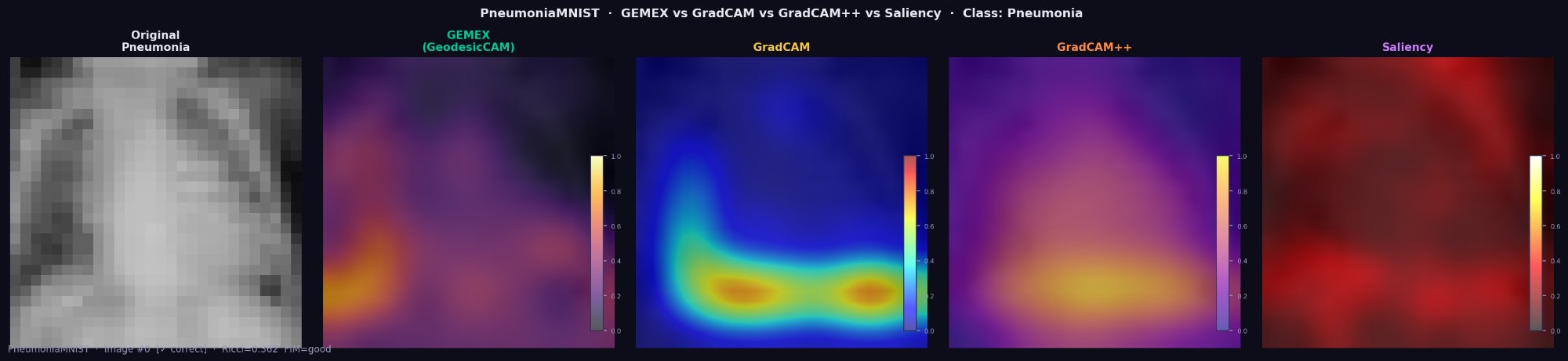
GEMEX (GeodesicCAM) identifies bilateral lower lobe infiltrates in this pneumonia
case using only predict_proba(). GradCAM requires full internal CNN access.
Deletion AUC: GEMEX=0.835, GradCAM=0.939, GradCAM++=0.708.
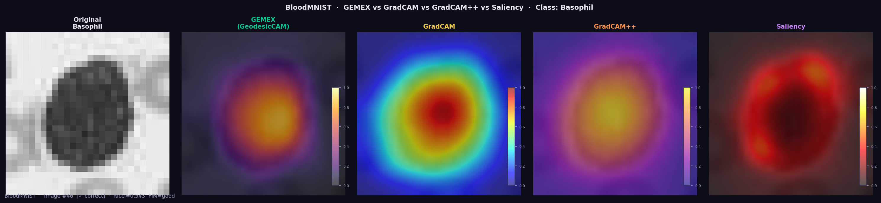
BloodMNIST is a 3-channel RGB dataset (blood cell microscopy, 8 cell types). For the Basophil class, GEMEX highlights the cell body as the dominant region (Ricci=0.545, FIM=good) — matching GradCAM and GradCAM++ — using only output probabilities, with no CNN layer access.
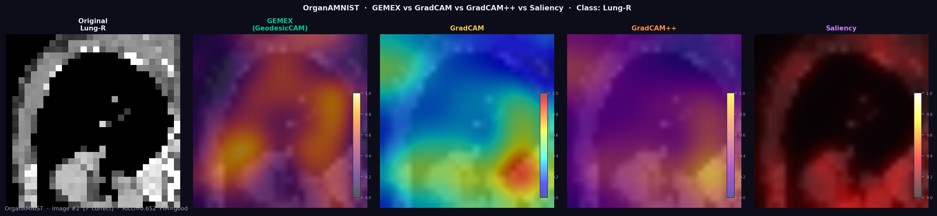
GEMEX achieves mean Deletion AUC of 0.335 across 11 organ classes, outperforming GradCAM (0.291) and Saliency (0.234). Mean Ricci scalar: 0.637±0.100 (all FIM quality ratings: good).
Important distinction: GradCAM treats CNNs as white boxes — it hooks into convolutional layer activations and backpropagates gradients. It cannot explain proprietary APIs, non-CNN models, or any model where internal layers are inaccessible. GEMEX explains the same CNN as a genuine black box.
GEMEX produces explanations that no other XAI library can generate, because it works from the geometry of the model's probability surface rather than from linear approximations or Shapley decompositions.
Capabilities exclusive to GEMEX:
- Reparametrisation-invariant attribution (GSF) — rescaling a feature never changes its attribution. SHAP values and LIME coefficients do not have this property.
- Holonomy-based pairwise interactions (PTI) — measures true nonlinear co-dependencies between features by parallel-transporting attribution vectors around closed loops on the manifold. SHAP interaction values and LIME coefficients capture only additive co-effects.
- Three-way Riemannian curvature (RCT) — the only XAI method that quantifies how a third feature modulates the interaction between two others, via the Riemann curvature tensor. No combination of pairwise methods can reproduce this.
- Manifold curvature per instance (Ricci scalar) — a single number that tells you how geometrically complex the model's decision surface is around each prediction. Higher Ricci = more curved = interpret with more care.
- Geometric uncertainty per feature — error bars on every attribution bar, derived from local manifold curvature. SHAP and LIME produce point estimates only.
- Feature Attention Sequence (FAS) — tracks which features the geodesic path passes through and for how long, revealing the model's internal geometric reasoning order. This temporal dimension of explanation does not exist elsewhere.
- Bias Trap Detection (BTD) — identifies features where the model spends disproportionate geometric attention relative to their actual effect, flagging potential confounders and spurious correlations before they reach a decision.
- Black-box image XAI across data types — explains CNN classifiers using only
predict_proba(), with no layer hooks or gradient access required. Works on greyscale, RGB, and mixed datasets. GradCAM requires full CNN architecture access.
# Tabular (medical, financial, scientific)
exp = Explainer(model, data_type='tabular', ...)

# Time series (ECG, HAR, sensor signals)
exp = Explainer(model, data_type='timeseries', ...)

# Image — patch-based, genuine black box (no architecture access)
cfg = GemexConfig(image_patch_size=4)   # 28×28 → 7×7=49 patches, ~6× faster
exp = Explainer(model, data_type='image', ..., config=cfg)pip install gemex # core
pip install gemex[torch] # + PyTorch CNN support
pip install medmnist # MedMNIST medical imaging
pip install gemex[full] # all backends| # | Script | Data type | Datasets |
|---|---|---|---|
| 01 | 01_tabular_heart_diabetes.py |
Tabular | Cleveland Heart Disease, Pima Diabetes (CSV files included) |
| 02 | 02_comparative_study.py |
Tabular | Heart + Diabetes + Breast Cancer vs SHAP/LIME/ELI5 (GBM, MLP, DeepMLP) |
| 03 | 03_timeseries_ecg.py |
Time series | ECG5000 (real data included in ECG5000/ folder) |
| 04 | 04_ablation_study.py |
Tabular | Per-component ablation with Wilcoxon tests |
| 05 | 05_statistical_comparison.py |
Tabular | Multi-seed study with bootstrap CI |
| 06 | 06_pneumoniamnist.py |
Image | PneumoniaMNIST — GEMEX vs GradCAM vs GradCAM++ |
| 07 | 07_pathmnist.py |
Image | PathMNIST — Colorectal cancer tissue (9 classes) |
| 08 | 08_dermamnist.py |
Image | DermaMNIST — Skin lesions HAM10000 (7 classes) |
| 09 | 09_organamnist.py |
Image | OrganAMNIST — Abdominal CT organs (11 classes) |
| 10 | 10_bloodmnist.py |
Image | BloodMNIST — Blood cell microscopy (8 classes, RGB) |
| 11 | 11_gemex_tabular_plots.py |
Tabular | Heart Disease — waterfall, heatmap, curvature plots |
| 12 | 12_triplet_hypergraph.py |
Tabular | Heart Disease — RCT three-way interactions hypergraph |
| 13 | 13_image_trio.py |
Image | PneumoniaMNIST / OrganAMNIST / BloodMNIST — standalone image_trio |
| 14 | 14_all_plots_showcase.py |
Tabular | Pima Diabetes — all 13 plot types in one run |
| Parameter | Default | Description |
|---|---|---|
n_geodesic_steps |
40 | 4th-order Runge-Kutta (RK4) integration steps along geodesic |
n_reference_samples |
80 | Background distribution sample size |
fim_epsilon_auto |
True | Auto-expand step size for tree/GBM models |
fim_local_n |
16 | Neighbourhood perturbation count |
interaction_order |
2 | 1=attribution only · 2=+PTI holonomy · 3=+RCT triplets |
image_patch_size |
1 | 1=pixel · 4=7×7 patches (~6× faster, stronger Ricci) |
model_type |
'auto' | 'auto' · 'tree' · 'smooth' |
gsf_normalise |
False | Force sum(GSF) = f(x) − f(baseline) |
Like any XAI framework, GEMEX involves trade-offs between geometric richness, computational cost, and axiomatic coverage. The points below are known limitations in v1.2.2 that are being actively addressed in future versions.
- Speed vs geometric richness: Tracing a geodesic requires more model calls per instance than straight-line perturbation methods such as SHAP or LIME. This is a fundamental trade-off of the manifold approach, not a fixable bug. See speed tips for settings that bring the cost down significantly. GPU parallelisation of the RK4 integrator is planned for v1.3.0.
- Tree model FIM quality: GBM, XGBoost and Random Forest produce flat
probability regions between split boundaries, making FIM gradient estimation
harder. GEMEX handles this automatically with adaptive step-size expansion,
though results are less reliable than on smooth models. Always check
result.fim_quality— a'poor'rating signals that Ricci scalar values for that instance should be treated with caution. Improved tree-specific FIM estimation is on the roadmap. - Completeness is a diagnostic, not a constraint: GEMEX attributions are not forced to sum to f(x) − f(baseline). Ablation testing confirmed that adding this constraint destabilises the geodesic. Completeness error is best treated as a descriptive metric rather than a quality gate. Future versions may explore optional soft-completeness modes.
- High-dimensional Ricci estimation: Beyond roughly 100 input features,
FIM neighbourhood sampling can become sparse and Ricci may return zero for
some instances. Increasing
fim_local_nandfim_local_sigmamitigates this in most cases. A more scalable high-dimensional FIM estimator is planned for v1.3.0.
GEMEX trades computation for geometric richness. Here are the main levers:
| Goal | Setting | Effect |
|---|---|---|
| Quick exploration | n_geodesic_steps=8, n_reference_samples=20 |
~5× faster, slightly less accurate geodesic |
| Attribution only | interaction_order=1 |
Skip PTI/RCT computation, saves ~30% |
| Image data | image_patch_size=4 |
784 pixels → 49 patches, ~6× faster |
| Tree models | model_type='tree' |
Starts at larger epsilon, avoids wasted zero-gradient calls |
| Production | n_geodesic_steps=12, n_reference_samples=30, interaction_order=1 |
~0.25 s/instance |
# Fast settings for exploration
cfg_fast = GemexConfig(
    n_geodesic_steps    = 8,
    n_reference_samples = 20,
    interaction_order   = 1,   # attribution only — no interactions
    verbose             = False
)

# Recommended settings for publication-quality results
cfg_full = GemexConfig(
    n_geodesic_steps    = 20,
    n_reference_samples = 60,
    interaction_order   = 2,   # + PTI pairwise interactions
    fim_local_n         = 16,
    fim_local_sigma     = 0.10,
)
FIM quality check: Always inspect result.fim_quality after explaining.
If it returns 'poor', increase fim_local_n or fim_local_sigma, or switch
to model_type='tree' for tree-based models.
result = exp.explain(x, X_reference=X_train)
if result.fim_quality == 'poor':
    print("Warning: FIM poorly estimated. Try increasing fim_local_n.")
    print(f"  Ricci scalar may be unreliable: {result.manifold_curvature:.4f}")
Batch explanation: Use explain_batch rather than looping for efficiency:
# Preferred — single reference computation
batch = exp.explain_batch(X_test[:50], X_reference=X_train)
fig = batch[0].plot('beeswarm', batch_results=batch, theme='dark')Kose, U. (2026). GEMEX: Model-Agnostic XAI via Geodesic Entropic Manifold Analysis. 8th International Congress on Human-Computer Interaction, Optimization and Robotic Applications (ICHORA 2026), May 21–23, 2026. Accepted. IEEE indexed.
The peer-reviewed paper presents full experimental validation: 5-seed comparative study (GBM, MLP, DeepMLP) across three medical datasets, ablation analysis, ECG5000 time series evaluation, and image XAI comparison with GradCAM and GradCAM++ on PneumoniaMNIST, OrganAMNIST and BloodMNIST (RGB).
@inproceedings{kose_gemex_2026,
  author    = {Kose, Utku},
  title     = {GEMEX: Model-Agnostic XAI via Geodesic Entropic Manifold Analysis},
  booktitle = {8th International Congress on Human-Computer Interaction,
               Optimization and Robotic Applications (HORA 2026)},
  year      = {2026},
  month     = {May},
  note      = {Accepted. IEEE ICHORA 2026. ORCID: 0000-0002-9652-6415}
}- Amari, S. & Nagaoka, H. (2000). Methods of Information Geometry. American Mathematical Society.
- Rao, C.R. (1945). Information and accuracy in statistical estimation. Bulletin of the Calcutta Mathematical Society, 37, 81–91.
- Kobayashi, S. & Nomizu, K. (1963). Foundations of Differential Geometry. Interscience.
- Alvarez-Melis, D. & Jaakkola, T.S. (2018). Towards Robust Interpretability with Self-Explaining Neural Networks. Advances in Neural Information Processing Systems 31 (NeurIPS 2018), 7786–7795.
- Luss, R., Chen, P.Y., Dhurandhar, A., Sattigeri, P., Zhang, Y., Shanmugam, K. & Tu, C.C. (2019). Generating Contrastive Explanations with Monotonic Attribute Functions. arXiv:1905.12698. Published KDD 2021, 1139–1149.
- Sundararajan, M., Taly, A. & Yan, Q. (2017). Axiomatic Attribution for Deep Networks. Proceedings of the 34th ICML, PMLR 70:3319–3328.
- Lundberg, S.M. & Lee, S.I. (2017). A unified approach to interpreting model predictions. NeurIPS 2017, 4765–4774.
- Ribeiro, M.T., Singh, S. & Guestrin, C. (2016). "Why should I trust you?". KDD 2016, 1135–1144.
- Yang, J. et al. (2023). MedMNIST v2. Scientific Data, 10(1), 41. https://doi.org/10.1038/s41597-022-01721-8
- Chattopadhay, A. et al. (2018). Grad-CAM++. WACV 2018, 839–847. https://doi.org/10.1109/WACV.2018.00097
MIT License · Copyright © 2026 Prof. Dr. Utku Kose
GEMEX was developed through a human-AI collaboration. The theoretical framework, mathematical foundations, algorithmic design decisions, and research directions are the original intellectual contribution of Prof. Dr. Utku Kose. AI-assisted tools were used in implementation and documentation phases.