Workflow for Spatial Transcriptomics datasets

by Younginn Park

This project implements the Visium HD Multi-sample Analysis workflow from 10x Genomics, based on their Guide and Colab Notebook, transformed into a reproducible workflow that can be executed across different environments.

The datasets used in this Analysis Guide are publicly available from 10x Genomics:

Human Colon Cancer and Normal Adjacent Datasets

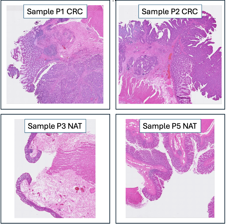
Sample tissues

The specific datasets used here are:

• Visium HD, Sample P1 Colon Cancer (CRC): Human colon cancer tissue (Patient 1).
• Visium HD, Sample P2 CRC: Human colon cancer tissue (Patient 2).
• Visium HD, Sample P3 Normal Adjacent Tissue (NAT): Normal adjacent human colon tissue (Patient 3).
• Visium HD, Sample P5 NAT: Normal adjacent human colon tissue (Patient 5).

If you are working with your own data, for each dataset, the outs directory will contain the cell segmentation based binned output and spatial output data. For a more detailed description of Visium HD's outputs, see the documentation on 10x Genomics website.

The data was originally processed using spaceranger count v3.0.0. However, to generate the Space Ranger cell segmentation outputs used in this project, the public colon cancer and normal adjacent tissue datasets were reprocessed using spaceranger count v4.0.1.

Usage

Clone repository

git clone https://github.com/young-sudo/spatialflow.git

Install Nextflow

# Download Nextflow
curl -s https://get.nextflow.io | bash

# Make Nextflow executable
chmod +x nextflow

# Move Nextflow into an executable path
mkdir -p $HOME/.local/bin/
mv nextflow $HOME/.local/bin/

# Confirm Nextflow is installed correctly
nextflow info

Basic run

nextflow run main.nf \
  -profile conda

Available profiles:

• standard - locally without containers
• conda - with default mode and Conda environment
• docker - with Docker
• singularity - with Singularity/Apptainer
• slurm - with slurm on HPC

For usage help run

nextflow run main.nf --help

Methods and Results

In order to download the same dataset as the one used in this analysis run:

!wget  https://cf.10xgenomics.com/supp/spatial-exp/analysis-workshop/multisample_raw_data.tar.gz
!tar xvzf multisample_raw_data.tar.gz
!rm multisample_raw_data.tar.gz

The SpatialData Object and Its Components

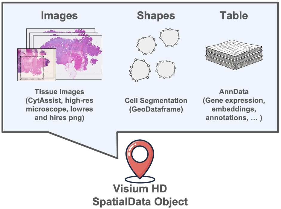
The spatialdata library is built to manage and analyze multiomic spatial datasets. It brings together multiple data types into a single, unified SpatialData object. These objects act as on-disk containers that utilize the Zarr file format to store various Elements or data types. A SpatialData object created from Visium HD data typically has the following Elements:

• Images: CytAssist and microscopy images (e.g., H&E, fluorescence) providing spatial context. These can be accessed via sdata.images.
• Shapes: Geometric annotations such as polygons or circles representing regions of interest, cells, or spots. In Visium HD, these often represent binned regions or cell segmentations. These are accessible via sdata.shapes.
• Tables: An AnnData object associated with the spatial elements, typically containing gene expression data, cellular metadata, and computational results (e.g., clusters, UMAP embeddings). This Element is used for downstream analyses and is accessed via sdata.tables. Each AnnData table within sdata.tables has:
  • .X: The primary data matrix (e.g., raw counts, normalized counts).
  • .obs: Observation metadata (e.g., sample ID, cluster assignments).
  • .var: Variable metadata (e.g., gene names).
  • .obsm: Multi-dimensional annotations (e.g., PCA, UMAP embeddings).
  • .layers: Alternative representations of .X.

In this project, the SpatialData object is created from the Zarr files. Each Zarr file is read into a list of SpatialData objects using the read_zarr function before the objects are concatenated. In addition, a sample column is added to each AnnData table within the SpatialData object, and the var_names_make_unique function is used to ensure that gene names are unique.

Clustering and Visualization

Scanpy's neighbors function generates a neighbor distance matrix and a neighborhood graph, which is used by Scanpy's leiden function to cluster the data. Finally, Scanpy’s umap function is used to visualize the results.

Clustering options in Scanpy

When running Scanpy's neighbors function, the distance metric selected will impact the clustering results. Therefore, you may need to explore different metrics depending on your datasets. Common distance metrics available in Scanpy include:

• Euclidean distance: The straight-line distance between two points in multi-dimensional space. It tends to group cells with similar overall expression magnitudes. If some genes have very high expression, they can dominate the distance calculation.
• Manhattan distance (L1 distance, City Block distance): The sum of the absolute differences of their coordinates. It is less sensitive to outliers than Euclidean distance. It is useful when differences in individual features are more important than overall magnitude.
• Cosine distance/similarity: Measures the angle between two vectors. A smaller angle (closer to 0) indicates higher similarity. It focuses on the orientation of the expression profiles, rather than their magnitude. This is particularly useful when the relative proportions of gene expression might be more informative than the absolute counts. Cell segmentation bins expressing the same genes in similar proportions will be considered close, even if one has a higher total count.
• Correlation-based distances (e.g., Pearson, Spearman): These typically define distance as 1 - correlation_coefficient. Cell segmentation bins are considered similar if their gene expression profiles are highly correlated, regardless of absolute expression values. This method identifies cell segmentation bins with similar patterns of gene activity.

A metric that emphasizes magnitude (like Euclidean) might connect cells based on overall transcriptional activity, while a metric emphasizing shape (like Cosine) might connect cells with similar gene expression patterns, even if their total RNA content differs.

For this analysis, Scanpy's correlation distance metric is used, and the clustering resolution (RES) is set to 0.8, and the number of neighbors is set to 15. These parameters will likely need to be fine-tuned for new analyses: a smaller resolution generally leads to fewer clusters, while increasing the number of neighbors will have a similar effect.

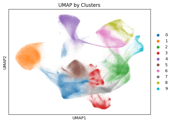
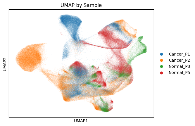
UMAP visualizations of cells, colored by clusters and sample

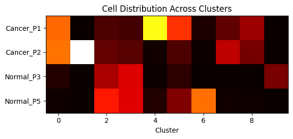
Cell distribution across clusters

Spatial cell annotations

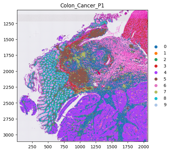
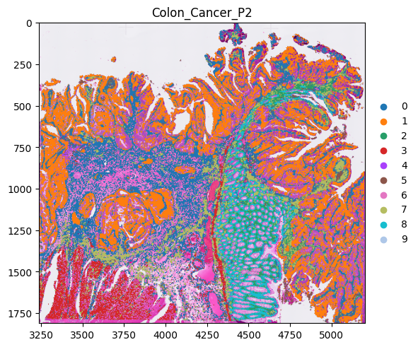
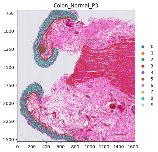
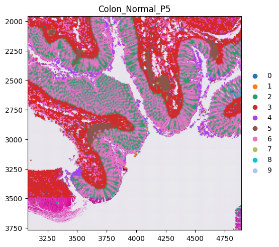
Sample tissues colored by cell clusters

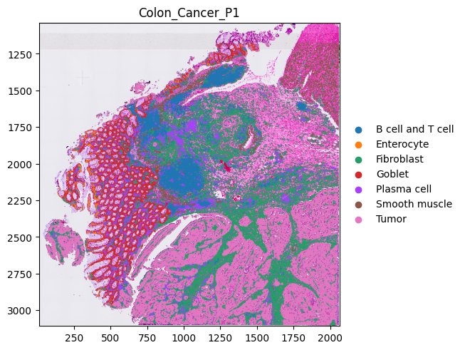
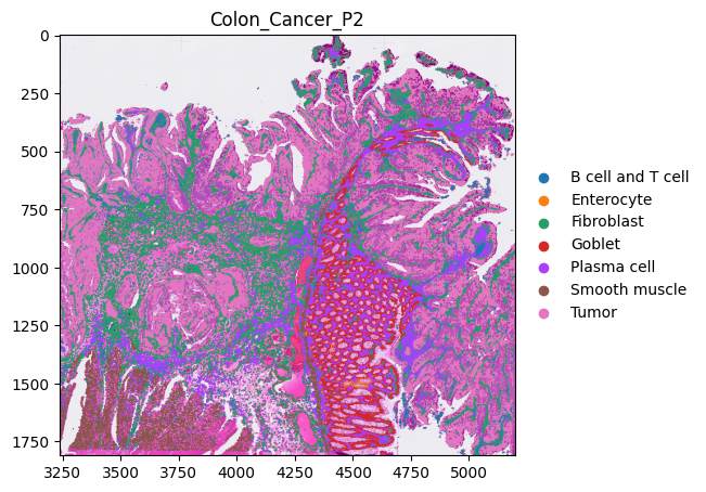
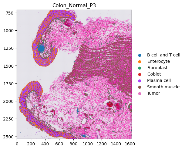
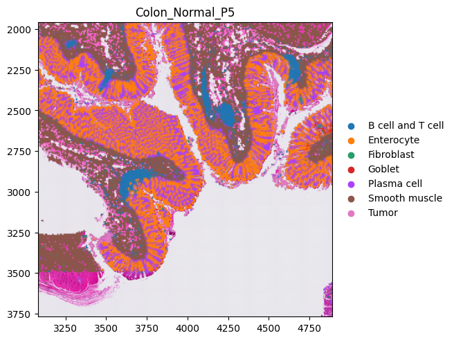
Sample tissues colored by cell annotations

Marker gene identification

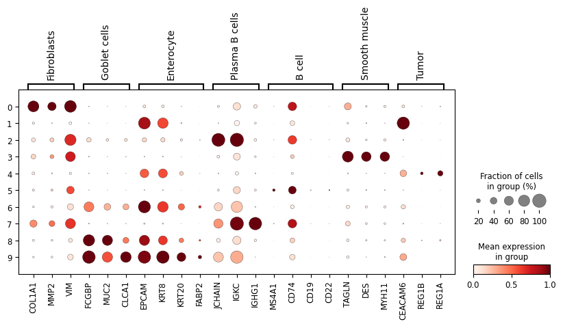
Canonical marker genes in clusters

Using the canonical markers, it can be observed that Cluster 3 expresses smooth muscle markers.

Cluster annotation can often be challenging when only canonical markers are used. To assist in this process, Scanpy’s rank_genes_groups function can be used to identify marker genes for each cluster. The results can be ranked by marker score or by the log fold-change. The top-ranked genes within each cluster can then be further analyzed using tools like Enrichr to infer the cluster's potential cell type.

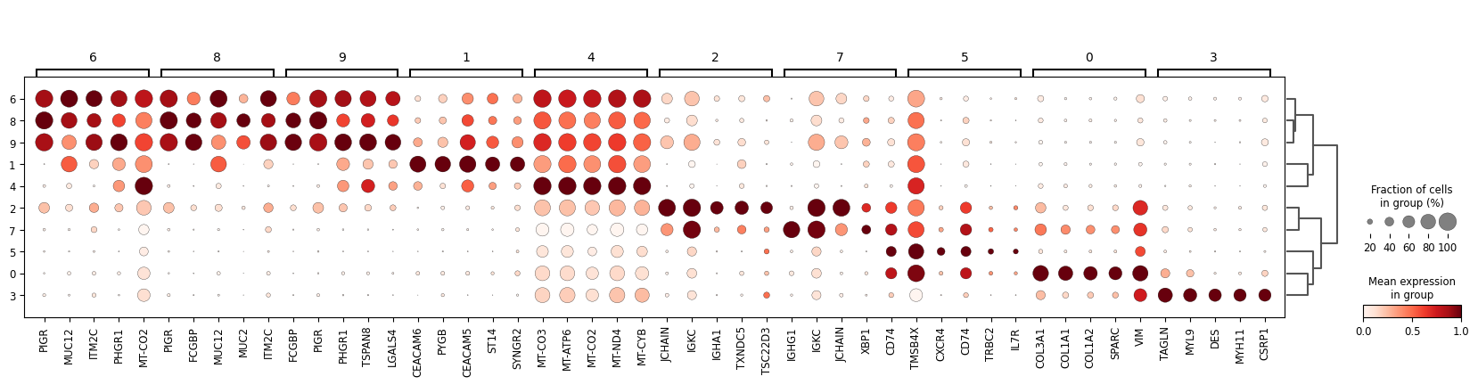
Marker genes ranked by Scanpy

Discussion

Upregulation of these genes in fibroblasts contributes to colon cancer progression by remodeling the extracellular matrix (ECM), secreting pro-tumorigenic factors, and fostering an immunosuppressive and pro-invasive tumor microenvironment.

Extracellular Matrix (ECM) Remodeling and Adhesion

These genes are directly involved in building, modifying, and interacting with the ECM.

• COL1A1, COL8A1, COL12A1: These genes encode different types of collagen, a major structural protein of the ECM. Cancer-associated fibroblasts (CAFs) produce excessive amounts of collagen, leading to a stiff and dense tumor stroma (desmoplasia). This dense matrix physically promotes cancer cell invasion and migration.
• COMP (Cartilage Oligomeric Matrix Protein): A non-collagenous protein of the ECM that helps organize other matrix components, contributing to the structural changes in the tumor.
• ADAM12 (ADAM Metallopeptidase Domain 12): This gene encodes a protein with both cell adhesion and protease functions. It can cleave ECM proteins, allowing cancer cells to move through the tissue more easily.
• ITGA11 (Integrin Subunit Alpha 11): An integrin protein that acts as a cell surface receptor. It helps fibroblasts adhere to and remodel collagen, a critical step in tumor matrix reorganization.
• ITGBL1 (Integrin Beta Like 1): This protein modulates cell-ECM adhesion and signaling, influencing cell migration and survival.

Signaling and Growth Factor Regulation

These genes are involved in signaling pathways that regulate cell proliferation, differentiation, and communication within the tumor microenvironment.

• SFRP4 (Secreted Frizzled-Related Protein 4): A modulator of the Wnt signaling pathway, which is often dysregulated in cancer. SFRP4 can promote tumor progression and metastasis.
• INHBA (Inhibin Beta A): A subunit of activin A, a growth factor that can activate fibroblasts, leading to the pro-tumorigenic desmoplastic reaction.
• CTHRC1 (Collagen Triple Helix Repeat Containing 1): A secreted protein that promotes cell migration and ECM remodeling. It is highly expressed in CAFs and is a known contributor to cancer cell invasion and a marker for poor prognosis.

We can now visualize the spatial expression of these genes.

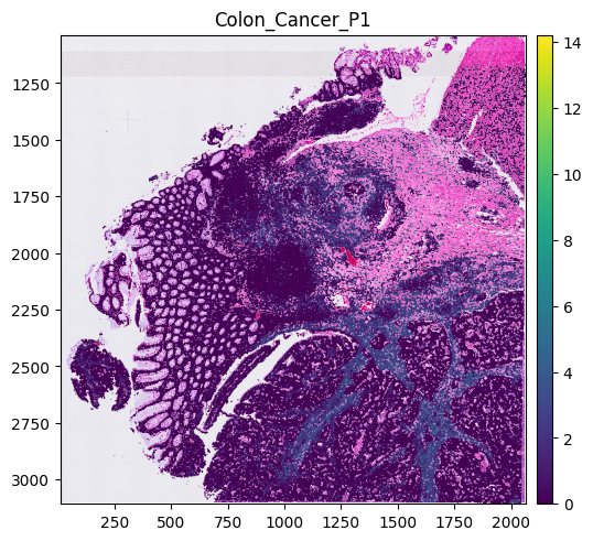
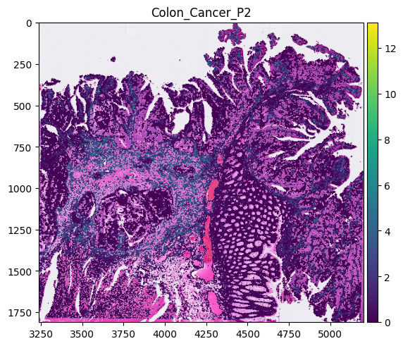
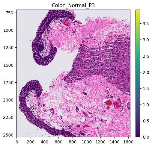
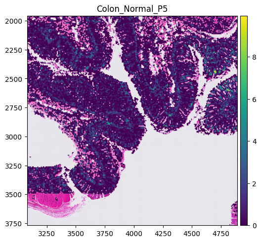
Plots for COL1A1's spatial gene expression in samples

COL1A1 is expressed by fibroblasts situated closer to the tumor in the Cancer samples. To delve deeper into the specific biology of these fibroblasts, the next step would involve subsetting the fibroblast-containing cluster from the overall dataset. This isolated subset can then be re-clustered to further investigate differences and heterogeneity within the fibroblast populations.

References

For additional resources on plotting SpatialData objects, see Spatialdata's Visium HD technology-focused tutorial.

For more detailed information on DESeq2 and setting up designs for various studies, see the official DESeq2 R documentation and Python documentation.