Gen3 Investigations
2021-12-17 Testing DRP pipetask throughput as a function of node occupancy on Perlmutter, Cori, and SDF
This post used lsst_distrib w_2021_42 for Perlmutter and SDF, and lsst_distrib w_2021_48 for Cori-KNL and Cori-Haswell.
The goal of these tests are to see what the throughput for processing DRP pipetask jobs is as a function of the number of concurrent processes. Ideally, if the occupancy is less than one process per core, the throughput should scale with the number of processes. However, we expect that resource contention can affect that scaling, even for # processes < # cores.
To test this on the NERSC machines, the isr task was run on DC2 raw files, using the command lines produced by the Gen3 middleware QuantumGraph, but using the python multiprocessing and subprocess modules directly to execute the jobs so that the number of concurrent jobs could be controlled precisely and to avoid known overheads and scheduling inefficiencies from using Parsl to control the workflow.
For comparison, the isr task was run on BOT data on the SDF cluster at SLAC. These machines are configured very similarly to the phase 2 Perlmutter CPUs, except that they have Rome processors instead of Milan. Phase 1 Perlmutter CPUs only have 64 cores and 256 GB memory, while the SDF CPUs have 128 cores and 512 GB, so this allowed the study to extend the occupancy per node by a factor of 2. One difference is that there are no calibration products for the BOT data, so the isr task is much simpler than for the DC2 data, lacking, in particular, B/F correction, which increases both the memory usage and execution time. Despite the fact that the BOT isr tasks ran ~3 faster and used a factor ~2 less memory per job, the scaling as a function of node occupancy is basically the same as for Perlmutter phase 1 up to 64 processes per node.
Here are the results:

The plot on the left shows the median elapsed (wall) time for the isr jobs to run as a function of # concurrent processes per node for each of the 4 platforms considered. The elapsed times were measured using the bash time command. Ideally, these curves should be flat as a function of # concurrent processes. The plot on the right shows the same data except with throughput (= # concurrent processes/median elapsed time) plotted versus # concurrent processes. The dotted curves show the ideal linear scaling of throughput with # concurrent processes. The measured curves deviate significantly from the ideal scaling for >64 processes, and seem to plateau to a constant throughput for the SDF case. The worst case, as inferred from the high end of the measured SDF curve, is a factor ~3 reduction in throughput relative to the linear scaling.
This post uses lsst_distrib w_2021_38
As of w_2021_38, the DIA part of the DRP pipeline appears to be largely complete. Just including the DIA-relevant tasks of the whole DRP pipeline, the high level task-only DAG is
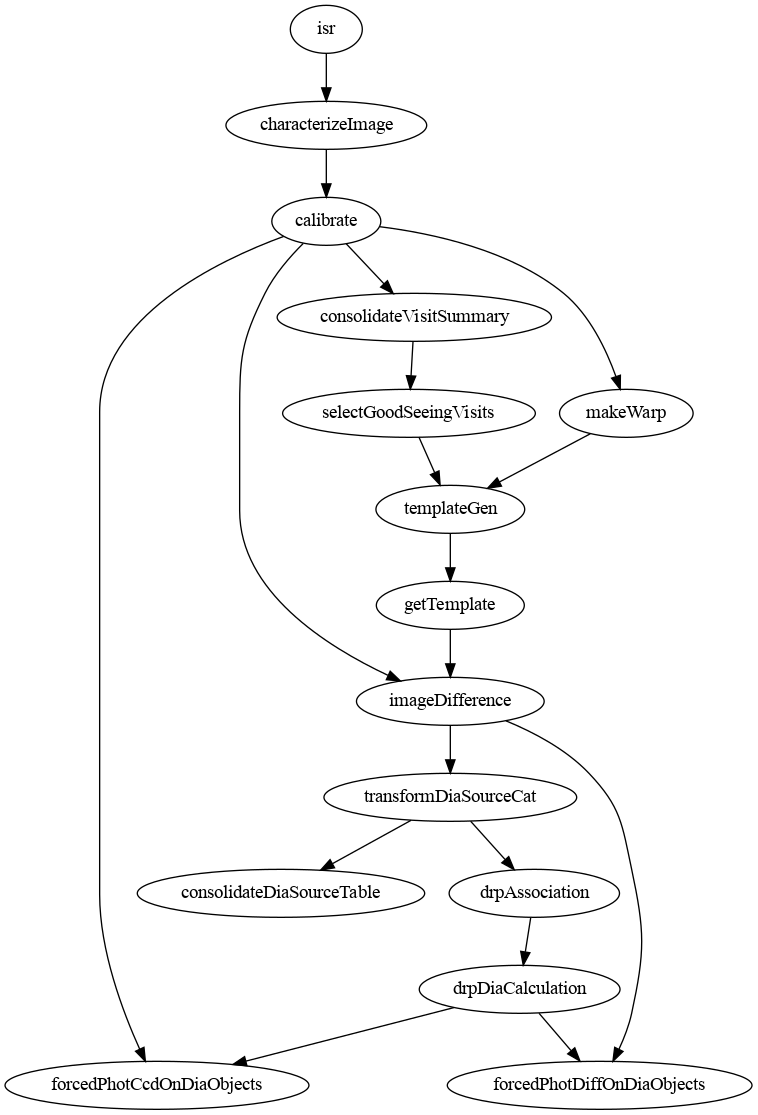
I've run this pipeline on the DC2 Run2.2i five-year depth data for tract 4638, patch 24 (this is one of the 6 tracts included in the DC2-DIA SNe analysis); and as for the tract 3828 WFD Y1 data, I've gathered cpu time and memory requirements for that pipeline running on Cori-Haswell. Here are some plots of the distributions of required resources for some selected tasks:
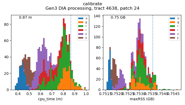
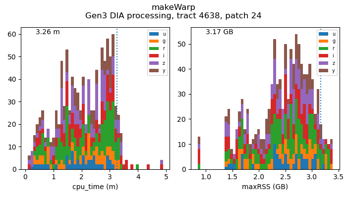
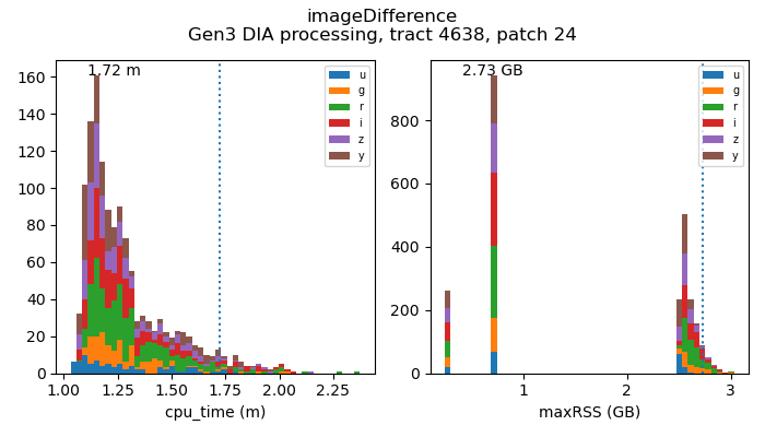
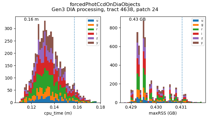
In each panel, the dotted vertical lines indicate the 95-th percentile value of the sample. That value is printed in the upper left corner and is used in the resource requirements for that task. Using those resource usage numbers, we can estimate the total computing time to process the 6 tracts considered in the DC2-DIA analysis for various platforms:
platform        cpu_factor    cores_per_node    memory_per_node   raw_node_hours
Cori-KNL           8                68                 96GB            19k
Cori-Haswell       1                32                128GB             3k
Perlmutter         1*              128                512GB            750
The Perlmutter entry assumes a cpu_factor = 1, i.e., the Gen3 pipetasks will use the same cpu time as on Cori-Haswell nodes. If we instead convert the Cori-Haswell raw execution time (3k hours) to NERSC hours and then to Perlmutter Node hours using the recommended conversion factor (dividing by 400), we get
(3000 raw Haswell)*(140 NERSC/raw Haswell)/(400 NERSC/Perlmutter Node) = ~1000 Perlmutter Node hours
This post uses lsst_distrib w_2021_38
This is a check that the BF kernels from the curated calibrations in obs_lsst_data, which are now installed in a repo via
butler write-curated-calibrations <repo> <instrument>
perform at least as well as the ones we generated ourselves from the raw flat pair calibration data. Here's the updated plot using the curated BF kernels:

This essentially just confirms work done in DM-30747.
This post uses lsst_distrib w_2021_33
Using the baseline_v2.0_10yrs.db cadence advertised at the 2021 PCW, here are the field pointings for the different proposalIds in the observations table:

We'll identify proposalId==1 as the WFD survey. I've simulated an observing sequence over the first year of WFD observations and computed the overlaps of sensor-visits with tracts and patches for the skymap we used for DC2. This information will give us the number of instances of each pipetask in the coadd/multiband part of the DRP pipeline, and that info will enable estimates of the computing resources--cpu time, memory per job, and disk space used--that are needed to support processing of Y1 WFD data. As we've seen below, for certain pipetasks, e.g., assembleCoadd, measure, forcedPhotCoadd, the required cpu time and memory per task instance depends on the number of visits in a given coadded patch. For this Y1 WFD survey simulation, here's the distribution of #visits/patch for each of the six LSST bands:

Combining the overlap information with the measurements of the cpu time and memory per task ascertained from running on Y1 tract 3828 DC2 data, along with average on-disk sizes of the various data products produced by each task, here are the estimates of resource needs for Y1 WFD:
            pipetask  num_instances     cpu_hours    max_GB    avg_GB    disk (TB)
0                isr       32825898  6.423604e+05  2.588478  2.588478  2866.919212
1  characterizeImage       32825898  1.233542e+06  0.828140  0.828140  3249.401350
2          calibrate       32825898  7.580443e+05  0.787716  0.787716  3406.132166
3           makeWarp       48457883  2.830984e+06  3.195480  3.195480  9484.062503
4      assembleCoadd        2695862  4.420030e+05  1.484659  1.477376   405.002744
5          detection        2695862  1.229541e+05  1.391117  1.214896   311.205865
6            measure        2695862  6.118123e+06  2.788095  1.808603   437.467370
7    forcedPhotCoadd        2695862  7.562931e+06  1.771112  1.564574   423.922747
8            deblend         449310  7.927732e+05  6.984100  6.984100    54.203169
Keeping all of the outputs, the disk space used by the DRP data products is ~21 PB. The input raw images for Y1 WFD are ~600 TB, so the coadd/multiband part of the DRP processing results in a factor ~35 increase over the raw data volume.
Assuming we can pack NERSC nodes as efficiently as possible, i.e., subject to memory constraints and requiring 1 core per process, we can estimate the node days needed to do the processing for Y1 WFD for the different platforms:
platform        cpu_factor    cores_per_node    memory_per_node   node_days
Cori-KNL           8                68                 96GB          198k
Cori-Haswell       1                32                128GB           28k
Perlmutter         1*              128                512GB            7k
Here the cpu_factor is an estimate of the relative execution time to run on a particular platform wrt the performance we measured on Cori-Haswell. We haven't yet profiled the DRP code on Perlmutter, so we take a value of 1.
This post uses lsst_distrib w_2021_21 and w_2021_22.
In order to estimate the computing needs for processing Y1 Rubin data, I've run the DRP pipeline on the DC2 Y1 tract 3828 data and gathered the maximum memory usage and cpu time for each task instance using the DC2 skymap, where each patch has the same pixel scale as the LSSTCam CCDs and approximately the same number of pixels, i.e., 4000 x 4000. Since using patches this large will result in excessively long task run times on Cori-KNL for some of the multiband tasks, I've run on Cori-Haswell instead.
For reference, here is the processing flow diagram for the DRP pipeline as of w_2021_23:

To give a sense of the scale of processing for a DC2 Y1 WFD patch, here's the workflow summary for the relevant tasks:
[cori04 cvmfs_w_2021_22] workflow_summary.py u/jchiang/sfp_3828/20210525T153432Z
task_type                    pending   launched    running  exec_done     failed   dep_fail      total
isr                                0          0          0       4676          0          0       4676
characterizeImage                  0          0          0       4676          0          0       4676
calibrate                          0          0          0       4673          3          0       4676
skyCorrectionTask                  0          0          0        188          0          0        188
consolidateVisitSummary            0          0          0        184          4          0        188
and here are the plots for the visit-level processing tasks, using w_2021_21:


The modes in the distributions of the memory usage by the isr, characterizeImage, and calibrate tasks suggest some dependence on the properties of the input images, but the overall distributions are sufficiently narrow that we can just take the upper end of the memory usage as a safe value for allocating task resources. The cpu time and memory for the skyCorrectionTask task actually scales with the number of CCDs being considered, with the full focal plane taking about 60 cpu minutes and 40GB of memory. The numbers are less that that for these tasks since only the CCDs from any given visit that covered the tract are included in this data set.
Here's the workflow summary for the coadd/multiband (and DIA) tasks:
[cori04 cvmfs_w_2021_22] workflow_summary.py u/jchiang/coadd_multiband_3828/20210531T215629Z
task_type                    pending   launched    running  exec_done     failed   dep_fail      total
makeWarp                           0          0          0       4527          1          0       4528
selectGoodSeeingVisits             0          0          0        294          0          0        294
assembleCoadd                      0          0          0        294          0          0        294
templateGen                        0          0          0        294          0          0        294
detection                          0          0          0        294          0          0        294
imageDifference                    0        167          0       4501          8          0       4676
mergeDetections                    0          0          0         49          0          0         49
deblend                            0          0          0         49          0          0         49
measure                            0          0          0        294          0          0        294
mergeMeasurements                  0          0          0         49          0          0         49
forcedPhotCoadd                    0          0          0        294          0          0        294
forcedPhotDiffim                 859        128         47       3604          0          8       4676
With the exception of the makeWarp and deblend tasks, the coaddition and multiband tasks have significant dependence on the number of visits. This dependence will be modeled in estimating the Y1 computing resource needs. The coadd and multiband tasks were run using w_2021_22:


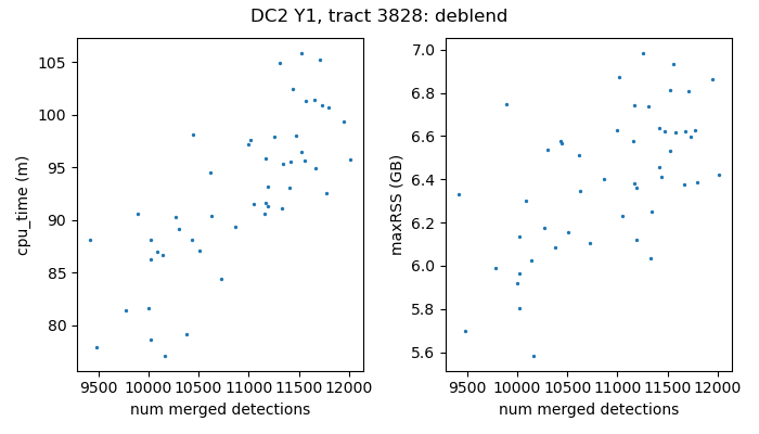
Note that the deblend task is the most resource intensive processing step. Furthermore, it operates on all six bands simultaneously, so it's a real choke point for the processing, with all of the upstream processing outputs and downstream processing inputs at the patch level flowing into and out of a single long-running, high memory footprint task. The cpu times and memory usage for the deblend task show somewhat stronger correlations when plotted versus the number of merged detections in each patch:
This post uses lsst_distrib w_2021_18.
We've used server-side connection pooling with pgbouncer to increase the number of connections that our postgres db can handle. Using settings of max_connections=128 for the postgres db and pool_mode=transaction, default_pool_size=128, max_client_conn=10000 for the pgbouncer configuration, we expect hoped to be able to support 10000 concurrent pipetask processes without overloading the database.
Here are some results of an initial small scale test with peak usage of ~2000 concurrent connections. This entailed running the Single Frame Processing tasks (isr, characterizeImage, calibrate, etc.) on ~3000 sensor-visits in the tract 4849-y1 data set using 20 Cori-KNL nodes. The number of tasks that can run per node is limited by the memory required by each task and the 96 GB capacity of the Cori-KNL nodes.

This is the time-history of concurrent tasks for all 20 nodes showing how the WorkQueueExecutor scheduled the execution of the various tasks as a function of wall time from the start of the processing.

And these are the distributions of wall-time duration for the different tasks.
Here are the results of a 100 node test with ~13000 sensor-visits. For characterizeImage tasks with ~1GB memory requirements, we'd expect (~90 GB/node)*(100 nodes)/(1 GB/task) ~ 9000 concurrent tasks.

Unfortunately, as the number of concurrent tasks exceed ~4000, we start seeing database connection errors:
  File "/opt/lsst/software/stack/conda/miniconda3-py38_4.9.2/envs/lsst-scipipe-0.5.0/lib/python3.8/site-packages/psycopg2/__init__.py", line 127, in connect
    conn = _connect(dsn, connection_factory=connection_factory, **kwasync)
psycopg2.OperationalError: ERROR:  no more connections allowed (max_client_conn)
The tasks labeled characterizeImage_err are the ones that reported these errors.
This post uses lsst_distrib w_2021_15.
I've created brighter-fatter kernels from the DC2 calibration flats using the photon transfer curve pipeline, cpPtc.yaml, and the brighter-fatter kernel pipeline, cpBfkSolve.yaml, which are available in w_2021_15.
To add the brighter-fatter kernels to a Gen3 DC2 repo at NERSC, they need to be imported first:
$ butler import <full path to gen3 repo> /global/cscratch1/sd/descdm/Gen3/dc2-bfk-calibs/dc2-bfk-calibs \
   --export-file /global/cscratch1/sd/descdm/Gen3/dc2-bfk-calibs/export_bfk_calibs.yaml
and then they need to be certified:
$ butler certify-calibrations <gen3 repo> shared/bfk/20210415T142710Z LSSTCam-imSim/calib \
    --begin-date 1980-01-01 --end-date 2050-01-01 bfk
The run name, shared/bfk/20210415T142710Z, must be used for these data. The calibration collection LSSTCam-imSim/calib is the one that is set up by default when converting a Gen2 repo with this script.
Running the equivalent of processCcd on a full (189 CCDs) DC2 i-band visit, both with and without the B/F correction enabled yields the following:

This shows the hexbin distributions of the PSF size (T = (base_SdssShape_xx + base_SdssShape_yy)*(0.2 arcsec)**2) for point-like sources with the brighter-fatter corrections applied (smaller hexbins, cyan points) and without them applied (larger hexbins, red points). The red and cyan points are the median values of T in bins centered on each point in psf_mag.
One notable feature of the processing is that the isr task requires ~2.6 GB of memory with the BF correction applied and only ~1.5 GB when it is disabled.
This post uses lsst_distrib w_2021_14.
Parsl's WorkQueueExecutor will use client-provided information on the resources needed for each task (memory usage, cores required, and disk space used) to automatically run in parallel as many tasks as possible on the available nodes. We have a work_queue-based Parsl config that runs on the Cori-KNL nodes at NERSC, and to use it, one needs to install the ndcctools software (which provides the work_queue module) as well as a development version of Parsl.
For running at NERSC with the lsst_distrib builds available on cvmfs, I create a local conda environment that can be "stacked" on top of the lsst_distrib conda environment. Here are the installation steps:
Set up a recent distribution of the stack:
$ LSST_DISTRIB=/cvmfs/sw.lsst.eu/linux-x86_64/lsst_distrib/w_2021_14
$ source ${LSST_DISTRIB}/loadLSST.bash
Specify a directory for the local conda environment:
$ wq_env=`pwd -P`/wq_env
Create the local environment for ndcctools and parsl:
$ conda create --prefix ${wq_env}
Activate the new environment, stacking it on top of the current environment:
$ conda activate --stack ${wq_env}
Install a version of ndcctools compatible with the python version (3.8) in the stack:
$ conda install -c conda-forge ndcctools=7.2.6=py38h4630a5e_0 --no-deps
The --no-deps option is needed to prevent conda from installing different versions of python as well as several other packages. The above distribution seems to work fine with the python environment that's included with lsst_distrib w_2021_14. If a different version of ndcctools is needed, the available ones can be seen with
$ conda search -c conda-forge ndcctools
Install the development version of parsl in the same area:
$ pip install --prefix ${wq_env} 'parsl[monitoring,workqueue] @ git+https://github.com/parsl/parsl@lsst-dm-202103'
Update the PYTHONPATH and PATH environment variables as needed:
$ export PYTHONPATH=${wq_env}/lib/python3.8/site-packages:${PYTHONPATH}
$ export PATH=${wq_env}/bin:${PATH}
The results shown in this post used lsst_distrib w_2021_12.
To make the job run times more manageable on the KNL batch queues, I've used patch sizes, 2000x2000 pixels, that are a factor 4 smaller than the patches in the standard DC2 skymap. Because of problems loading an all-sky skymap with 4 times as many patches into a postgres-based registry, I used a DiscreteSkyMap, made with this config, that just encloses the DC2 WFD region:


The figure on the left shows the full, single tract for this DiscreteSkyMap, and the figure on the right shows a zoom in on DC2 tract 3828, which is the region covering the data considered here. The red rectangles are the 7x7 patches covering tract 3828, and the blue rectangles are a subset of patches from the single tract in the DiscreteSkyMap.
Here are some memory usage for various coaddition/multiband processing tasks.

Modulo the outliers at low numbers of visits for the assembleCoadd and detection tasks, this should be sufficient get rough estimates of the needed memory usage to use with the Parsl WorkQueueExecutor.
The work in this post used lsst_distrib w_2021_08 for doing the single frame processing of the tract 3282 Y1 data and used lsst_distrib w_2021_11 for exporting the data from the old repo and setting up and importing into the new repo.
The data of interest are the outputs from running single frame processing so that they don't need to be regenerated when switching to a new weekly/repo. AFAIK, there's no general script or butler command to do this, so I wrote one for our special case. Here's the command I used to export those data from the w_2021_08 processing at NERSC:
$ python $GEN3_WORKFLOW_DIR/scripts/gen3_setup/export_drp_outputs.py gen3-3828-y1 --collections shared/sfp_3828_y1/20210223T191036Z \
      --export-file export_sfp_3828_y1.yaml
where the desired collection name is ascertained using the butler query-collections command.
I created the new Gen3 repo with w_2021_11:
$ butler create --seed-config butler_seed.yaml gen3-3828-y1
where butler_seed.yaml contains
datastore:
  checksum: false
  root: <butlerRoot>
registry:
  db: postgresql://db.postgres-desc-dev.dev-cattle.stable.spin.nersc.org:5432/desc_dm_gen3_spin
  namespace: <schema_name>
Here <schema_name> would be replaced by the name of the desired schema in the postgres db.
Using the convert_gen2-repo.py script, I converted one of our test Gen2 repos. That script will ingest the raw, CALIB, and ref cat files from the input repo; it will register the DC2 skymap; and it will set a default collection consisting of those inputs:
$ python $GEN3_WORKFLOW_DIR/scripts/gen3_setup/convert_gen2-repo.py /global/cscratch1/sd/descdm/Gen3/Gen2_repos/tract_3828_y1 gen3-3828-y1
Importing the data exported from the original (w_2021_08-based) repo is a single butler command:
$ butler import <full_path_to_new_repo> <full_path_to_old_repo> --export-file <full_path_to_export_file>
Using full paths here is recommended by the DM team.
The examples in this post use lsst_distrib w_2021_08 and lsst_distrib v19.0.0
Here cpu times and maximum RSS values for the coadd/multiband pipeline tasks run on Run2.2i Y1 DC2 for tract 3828:

These data were extracted from the repo metadata that stored for some of the pipeline tasks. Note that only the first 20 patches that finished are included in these data. The other 29 patches aren't fully processed and probably contain more visits per patch, which would yield longer run times for the all of these tasks.
Gen2 DRP processing also stores these metadata, so I've scrapped the tract 3828 values from the descdm DR2 repo at NERSC, /global/cscratch1/sd/descdm/DC2/DR2/repo:
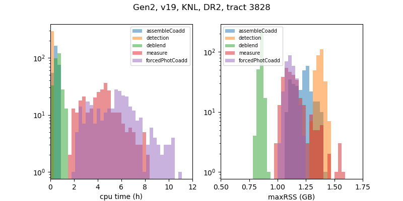
Note that both of these datasets were processed on Cori-KNL nodes. Extracting the same stats for 3828 from the performance runs I did on Cori-Haswell shows similar memory footprints, but about a factor ~6 shorter cpu times:

Checkpointing isn't available for single quanta tasks, so the long cpu times of ~10 hours are problematic for running in the NERSC batch queues with Parsl. To make these jobs more manageable, Jim B suggests using smaller patches. This can be set in the makeSkyMap.py config file.
The examples in this post use lsst_distrib w_2020_44.
As noted below, one can decompose a QuantumGraph into nodes/quanta that correspond to individual, concrete instances of tasks like ISR, deblending, or forced photometry on specific input data. Since the Gen3 code computes the expected inputs and outputs of each of these task instances, one can form a detailed DAG for every processing instance and data product in a particular pipeline processing of an input dataset. One can use that DAG to with a "workflow engine" to manage the execution of such a pipeline for a given set of computing resources. The ctrl_bps package does that using HTCondor/DAGMan- and Pegasus-based workflow engines.
Based on the ctrl_bps implementation, I've written a lighter weight module, task_graph.py, that has similar basic functionality while allowing me to see how a very simple Parsl-based implementation might work.
The key component of this module is the Task class, which holds the execution information for a given quantum in a Gen3 QuantumGraph, i.e., the pipeline task to run and its input and outputs. Following what's done in ctrl_bps, that quantum can be persisted to a pickle file on disk and then executed with a generic pipetask run --qgraph <filename> command line. For running in Parsl, we just need to wrap that command line as a bash_app:
@parsl.bash_app
def run_quantum(task, inputs=(), stdout=None, stderr=None):
    """
    Run the quantum associated with the specified task.
    If the task's outputs are present in the repo, it's done so
    return an empty string as a no-op command line.
    """
    if task.done:
        return ''
    return task.command_line()
where the Task.command_line function is defined as
   def command_line(self):
        """
        Write the QuantumGraph node associated with this task as a
        subgraph to a pickle file and generate the `pipetask run` command
        line to execute the subgraph.
        """
        config = dict(self.task_graph.config)
        config['quantum_file'] = self.write_subgraph()     # This line writes the pickle file.
        return '''time pipetask run -b %(butlerConfig)s \\
        -i %(inCollection)s \\
        --output-run %(outCollection)s --extend-run --skip-init-writes \\
        --qgraph %(quantum_file)s --skip-existing \\
        --no-versions''' % config
Each Task object has a list of prerequisite tasks, the Task.prereqs attribute; and with that one can define a Task.get_future() function that recursively creates the DAG that Parsl executes:
    def get_future(self):
        """
        Return the future of the run_quantum bash_app that is
        used to execute this task, collecting input futures from
        this task's prerequisite tasks.
        """
        if self.future is None:
            inputs = [_.get_future() for _ in self.prereqs]
            self.future = run_quantum(self, inputs=inputs, **self.log_files())
        return self.future
So if one has the Task object for a particular task in the pipeline instance, e.g., the ForcedPhotCoaddTask, one need only call its .get_future() method and Parsl will execute the parts of the DAG on which that task depends as well as the task itself.
Being able to work with the QuantumGraph and its quanta is an enormous simplification over the work that we are currently doing to keep track of the visits, filters, tracts, patches, etc. for each of the pipetasks in a Gen2-based DRP pipeline (see for example).
The examples in this post use lsst_distrib w_2020_43.
As Jim B. showed in his Rubin Operations Bootcamp tutorial, one can execute a pipeline by providing the --pipeline option to the pipetask run command. Alternatively, if one has a QuantumGraph pickle file, that file can be specified with the --qgraph option instead of the yaml definition:
$ pipetask run -b gen3-repo/ -i LSSTCam-imSim/raw/all,LSSTCam-imSim/calib,ref_cat,skymaps/imsim \
   --output-run shared/single_ccd_DRP --qgraph DRP_3828_24_177.pickle
ctrl.mpexec.cmdLineFwk INFO: QuantumGraph contains 11 quanta for 11 tasks
conda.common.io INFO: overtaking stderr and stdout
conda.common.io INFO: stderr and stdout yielding back
isr INFO: Converting exposure to floating point values.
isr INFO: Assembling CCD from amplifiers.
isr INFO: Applying bias correction.
isr INFO: Applying crosstalk correction.
isr.crosstalk INFO: Applying crosstalk correction.
<...>
Having the QuantumGraph for a given pipeline execution is useful since it provides access to the graph nodes that contain the individual quanta of processing tasks:
from lsst.daf.butler import DimensionUniverse
from lsst.pipe.base import QuantumGraph

qgraph_file = 'DRP_3828_24_177.pickle'
with open(qgraph_file, 'rb') as fd:
    qgraph = QuantumGraph.load(fd, DimensionUniverse())

nodes = list(qgraph)
for i, node in enumerate(nodes):
    print(i, node.taskDef)
This code snippet produces the following screen output:
0 TaskDef(IsrTask, label=isr)
1 TaskDef(CharacterizeImageTask, label=charImage)
2 TaskDef(CalibrateTask, label=calibrate)
3 TaskDef(MakeWarpTask, label=makeWarpTask)
4 TaskDef(CompareWarpAssembleCoaddTask, label=assembleCoadd)
5 TaskDef(DetectCoaddSourcesTask, label=detection)
6 TaskDef(MergeDetectionsTask, label=mergeDetections)
7 TaskDef(DeblendCoaddSourcesSingleTask, label=deblend)
8 TaskDef(MeasureMergedCoaddSourcesTask, label=measure)
9 TaskDef(MergeMeasurementsTask, label=mergeMeasurements)
10 TaskDef(ForcedPhotCoaddTask, label=forcedPhotCoadd)
We can look at each node to inspect the input and outputs, e.g.,
deblend_node = node[7]

print(deblend_node.taskDef)
print('Inputs:')
for key, value in deblend_node.quantum.inputs.items():
    print(f'{key}:')
    print('  ', value)
    print()

print()
print('Outputs:')
for key, value in deblend_node.quantum.outputs.items():
    print(f'{key}:')
    print('  ', value)
    print()
which produces
TaskDef(DeblendCoaddSourcesSingleTask, label=deblend)
Inputs:
DatasetType('deepCoadd_mergeDet', {skymap, tract, patch}, SourceCatalog):
   [DatasetRef(DatasetType('deepCoadd_mergeDet', {skymap, tract, patch}, SourceCatalog), {skymap: DC2, tract: 3828, patch: 24})]

DatasetType('deepCoadd_calexp', {band, skymap, tract, patch}, ExposureF):
   [DatasetRef(DatasetType('deepCoadd_calexp', {band, skymap, tract, patch}, ExposureF), {band: i, skymap: DC2, tract: 3828, patch: 24})]


Outputs:
DatasetType('deepCoadd_deblendedFlux', {band, skymap, tract, patch}, SourceCatalog):
   [DatasetRef(DatasetType('deepCoadd_deblendedFlux', {band, skymap, tract, patch}, SourceCatalog), {band: i, skymap: DC2, tract: 3828, patch: 24})]

DatasetType('deblend_metadata', {band, skymap, tract, patch}, PropertySet):
   [DatasetRef(DatasetType('deblend_metadata', {band, skymap, tract, patch}, PropertySet), {band: i, skymap: DC2, tract: 3828, patch: 24})]
This shows that the deblending task has two types of inputs, a SourceCatalog from the MergeDetectionsTask and ExposureF objects from the DectectCoaddSourcesTask; and two outputs, a SourceCatalog containing the deblended fluxes and a PropertySet containing metadata associated with the deblending. These same dependencies can be seen in the DAG shown below, but the point is that the interface provides programmatic access that can be used to control the execution of a pipeline.
One way to run individual quanta contained in a QuantumGraph would be to repackage the node containing a given quantum as a stand-alone QuantumGraph and write the associated pickle file. Let's do this for the IsrTask so that we can run it without needing any outputs from other parts of the DRP pipeline:
isr_node = nodes[0]

subgraph = qgraph.subset(isr_node)
with open('isr_quantum_3828_24_177.pickle', 'wb') as fd:
    subgraph.save(fd)
We can run this using pipetask run --qgraph as we did for the full QuantumGraph pickle file:
$ pipetask run -b gen3-repo/ -i LSSTCam-imSim/raw/all,LSSTCam-imSim/calib,ref_cat,skymaps/imsim \
>   --output-run shared/isr_test --qgraph isr_quantum_3828_24_177.pickle
ctrl.mpexec.cmdLineFwk INFO: QuantumGraph contains 1 quanta for 1 tasks
conda.common.io INFO: overtaking stderr and stdout
conda.common.io INFO: stderr and stdout yielding back
isr INFO: Converting exposure to floating point values.
isr INFO: Assembling CCD from amplifiers.
isr INFO: Applying bias correction.
isr INFO: Applying crosstalk correction.
isr.crosstalk INFO: Applying crosstalk correction.
isr INFO: Masking NAN value pixels.
isr INFO: Widening saturation trails.
isr INFO: Applying dark correction.
isr INFO: Applying flat correction.
isr INFO: Applying fringe correction after flat.
isr.fringe INFO: Filter not found in FringeTaskConfig.filters. Skipping fringe correction.
isr INFO: Interpolating masked pixels.
isr WARN: No rough magnitude zero point set for filter i.
isr INFO: Setting rough magnitude zero point: 31.692803
Persisting the individual quanta as separate QuantumGraph pickle files and executing those as pipetask run command lines appears to be the approach taken by the ctrl_bps "Batch Production Service" package. The execution of the pipeline is managed on the backend by a workflow engine implementation. The existing workflow engines use either Pegasus or HTCondor. For running at NERSC or similar sites, DESC may want to implement its own workflow engine to use with ctrl_bps, thereby insulating us from changes to the Gen3 interfaces.
In this post, we'll generate a QuantumGraph from a yaml pipeline definition using Gen3 tools that will run on DC2 data.
This will be done with lsst_distrib w_2020_43.
- Assuming
w_2020_43is set up, we clone a copy of theLSSTDESC/gen3_workflowrepo, checkout theu/jchiang/gen3_scriptsbranch and set it up:
$ git clone git@github.com:LSSTDESC/gen3_workflow.git
$ cd gen3_workflow
$ git checkout u/jchiang/gen3_scripts
$ setup -r . -j
- In our work area, we set up a small Gen2 test repo with DC2 data. For doing development and testing, it's probably better to ingest just enough data to cover a single patch in all six bands. This will mean 3-4 visits per band, covering the selected patch so that there are no unobserved regions from the inter-CCD gaps present in single visit data. Note that the flats in the Gen2 CALIB folder will need to be updated with physical filter names in order to work with recent
lsst_distribweeklies. Assuming the Gen2 repo is namedgen2-repo, we'll use thebutler createcommand to make a Gen3 repo to receive the converted data. By default, this will create a repo with an sqlite3-based registry file which should be sufficient for a small amount of data:
$ ls gen2-repo
CALIB  calibrations  _mapper  raw  ref_cats  registry.sqlite3
$ butler create gen3-repo
$ ls gen3-repo
butler.yaml  gen3.sqlite3
- Ideally, we should be able to use the
butler convertcommand to convert our Gen2 repo to a Gen3 version directly, but for now we'll use theconvert_repo.pyscript to convert the raw files, the calibs, and the reference catalogs. (The script will need some minor editing if the repos aren't calledgen2-repoandgen3-repo, respectively):
$ python $GEN3_WORKFLOW_DIR/scripts/gen3_scripts/convert_gen2-repo.py
Note that this script doesn't convert the brighter-fatter kernels in the gen2-repo/calibrations folder or the full sky-frame images in gen2-repo/CALIB/SKY folder. Those aren't needed for now to run the Gen3 processing.
- An existing skymap in the Gen2 repo could, in principle, be converted, but it's easier for now to simply create it from scratch. For this, we'll use the
gen3_workflow/config/makeSkyMap.pyconfig file. That config file is a slightly modified version of the one currently inobs_lsst/config:
$ makeGen3Skymap.py gen3-repo skymaps/imsim --config-file $GEN3_WORKFLOW_DIR/config/makeSkyMap.py
- At this point, there are various collections in
gen3-repo:
$ butler query-collections gen3-repo
collections:
- LSSTCam-imSim/raw/all
- LSSTCam-imSim/calib
- LSSTCam-imSim/calib/unbounded
- LSSTCam-imSim/calib/gen2/2022-08-06
- LSSTCam-imSim/calib/gen2/2022-01-01
- ref_cat
- skymaps/imsim
In gen3_workflow/pipelines, we have versions of the yaml files for the DRP pipeline that have been modified to work with DC2 data Specifically, they've been updated with the configs to map the physical filter names to the band names in the reference catalogs we're using:
$ cat $GEN3_WORKFLOW_DIR/pipelines/DRP.yaml
description: DRP
inherits:
  - location: $GEN3_WORKFLOW_DIR/pipelines/ProcessCcd.yaml
  - location: $GEN3_WORKFLOW_DIR/pipelines/Coaddition.yaml
  - location: $GEN3_WORKFLOW_DIR/pipelines/Multiband.yaml
  - location: $GEN3_WORKFLOW_DIR/pipelines/Forced.yaml

$ cat $GEN3_WORKFLOW_DIR/pipelines/ProcessCcd.yaml
description: ProcessCcd
instrument: lsst.obs.lsst.LsstImSim
tasks:
  isr: lsst.ip.isr.IsrTask
  charImage: lsst.pipe.tasks.characterizeImage.CharacterizeImageTask
  calibrate:
    class: lsst.pipe.tasks.calibrate.CalibrateTask
    config:
      file: $GEN3_WORKFLOW_DIR/config/calibration_filterMap.py

$ cat $GEN3_WORKFLOW_DIR/config/calibration_filterMap.py
DC2_filterMap = {f'{_}_sim_1.4': f'lsst_{_}_smeared' for _ in 'ugrizy'}
config.astromRefObjLoader.filterMap = DC2_filterMap
config.photoRefObjLoader.filterMap = DC2_filterMap
To generate a QuantumGraph for a single tract-patch combination, we use the pipetask qgraph command:
$ tract=3828
$ patch=24
$ pipeline=DRP

$ pipetask qgraph \
   -d "tract=${tract} AND patch=${patch}" \
   -i "LSSTCam-imSim/raw/all,LSSTCam-imSim/calib,ref_cat,skymaps/imsim" \
   -b gen3-repo \
   --instrument lsst.obs.lsst.LsstCamImSim \
   --pipeline ${GEN3_WORKFLOW_DIR}/pipelines/${pipeline}.yaml \
   --save-qgraph ${pipeline}_${tract}_${patch}.pickle \
   --qgraph-dot ${pipeline}_${tract}_${patch}.dot
py.warnings WARN: /opt/lsst/software/stack/stack/miniconda3-py37_4.8.2-cb4e2dc/Linux64/pipe_base/20.0.0-23-g8900aa8+dfd6ff4ddf/python/lsst/pipe/base/pipelineIR.py:331: UserWarning: Any instrument definitions in imported pipelines are ignored. if an instrument is desired please define it in the top most pipeline
  warnings.warn("Any instrument definitions in imported pipelines are ignored. "

ctrl.mpexec.cmdLineFwk INFO: QuantumGraph contains 368 quanta for 11 tasks
The resulting pickle file, DRP_3828_24.pickle, contains the QuantumGraph composed of the 368 quanta for the 11 separate tasks (e.g., IsrTask, CharacterizeImageTask, etc.) needed to process the data for tract 3828, patch 24. The file DRP_3828_24.dot contains a diagram depicting the DAG of that pipeline with all of the relationships between the tasks and their inputs and outputs. Even though the repo contains a tiny amount of data (~100 sensor-visits), rendering that DAG would make a rather large diagram. We can generate the DAG for the DRP processing of a single CCD for a specific visit by adding appropriate constraints to the data selection option:
$ pipetask qgraph \
   -d "tract=3828 AND patch=24 AND detector=177 AND visit=192355" \
   -i "LSSTCam-imSim/raw/all,LSSTCam-imSim/calib,ref_cat,skymaps/imsim" \
   -b gen3-repo \
   --instrument lsst.obs.lsst.LsstCamImSim \
   --pipeline ${GEN3_WORKFLOW_DIR}/pipelines/DRP.yaml \
   --save-qgraph DRP_3828_24_177.pickle \
   --qgraph-dot DRP_3828_24_177.dot
To make a png of the DAG, we run dot -Tpng DRP_3828_24_177.dot > DRP_3828_24_177.png:
