Repository navigation
Metrics aggregation and ranking
In one sentence: how 41 per-area sweeps become one EU-wide frontier, how each area's distance to its frontier becomes a few rankable numbers (and colours), and what the descriptive indicators of today's network measure.
Where this sits: at the end of the pipeline (GeoDMS → Arrow → Julia LP → sweep → rounding → scenarios → deck). Everything here except the descriptives is post-processing of
doc/deck_data.json; the descriptives come straight from GeoDMS. Nothing on this page solves an LP. Upstream: The lambda sweep and the Pareto frontier, Scenarios S1 S2 S3. Downstream: Deck and charts pipeline, Pharmacy results September 2026. Formal statement: §7 of Lambda sweep method.
All numbers are the state of commit e25416b (10 September 2026), with Italy still on the ESPON 2021 shapefile (12 991 pharmacies) rather than the OECD-geolocated Ministry-of-Health list (20 635; issue #53, whose regeneration is not in this checkout and changes the rankings — Branches data and environment). "pNN" is a slide of the 74-slide results deck doc/lambda_sweep5.pptx (76 slides after the unpushed 216ac77).
Counting the areas. 42 swept areas = 14 countries + 28 NUTS-1 regions; 41 in the aggregate (country-Poland dropped, below); 44 in ORDER and policy_typology.csv (Hungary and Finland entered ahead of their sweeps); the descriptives count 17 countries (14 + France, Italy, Sweden as wholes) and 25 NUTS-1 rows (NL, FR + 13, IT + 5, SE + 3).
The aggregate exists to put one EU-wide S1 and S2 on the deck (p59; commit d0ae5ef, 5 July 2026, marked "user request" — who asked is not recorded). Each area is swept on its own at a price λ per open location (λ = w · €100 000, the € a placeholder — The lambda sweep and the Pareto frontier, Glossary), minimising travel cost + λ · number of locations. The objective is separable — a sum of per-area objectives with no constraint linking two areas (a client in Estonia can never be assigned to a pharmacy in Austria) — so no joint solve is needed: at a common λ the sum of the per-area optima is the optimum of the combined problem, (Σ counts, Σ travel). Combining by count instead would mean comparing every way of splitting a total over 41 areas; a common price equalises the marginal value of a location everywhere and the split falls out by itself. The sum keeps both bounds: summed LP travel is still a certified floor (The facility location model explained); summed multistart networks are still buildable, hence a ceiling (From LP fractions to real pharmacies). Every area must therefore be swept on the same w-grid with no early stop — an early stop truncates the aggregate's range, as Belgium's at w = 0.1 did before commit 206923c (grid history on The lambda sweep and the Pareto frontier).
Each sweep row carries sum_y (the LP's fractional count), relax (LP travel, the lower bound), multi (multistart travel — the drawn frontier and upper bound), n_open (the multistart's integer count) and frac (how many y are fractional) — Log lines and output files. The 1-2-5 grid is common to all areas, but the #52 bisection runs (Scenarios S1 S2 S3) added area-specific w and some sweeps stop earlier. aggregate_fd in doc/build_charts.py (around line 228) therefore:
-
takes each area's rows with w > 0, sorted by w;
-
keeps only the range every area covers (
w_lo= the largest of the smallest w,w_hi= the smallest of the largest): [1e-4, 0.5] LINEAR, [1e-4, 0.02] LOGISTIC. The LOGISTIC ceiling is Denmark's alone (its sweep stopped at the July-era defaultw_max= 0.02, commit f93aea1, while every other area reaches 0.5), so 38 % of the LOGISTIC range solved elsewhere is discarded until Denmark is re-swept; -
forms the union of all distinct w in that range (68 points LINEAR, 56 LOGISTIC);
-
at each union w an area contributes its solved row if it has one, otherwise
_interp_at(around line 209) interpolates the five columns between its two bracketing rows linearly in ln w:$$f = \frac{\ln w - \ln w_{lo}}{\ln w_{hi} - \ln w_{lo}},\qquad v = v_{lo} + f,(v_{hi} - v_{lo})$$ In words: between two of its own grid points an area moves in a straight line against the logarithm of the price — log because the grid is geometric (half-way between w = 0.2 and 0.5 is 0.316, not 0.35). A union row only one area solved is partly synthetic; the chart draws it like any other. Why log-linear is not recorded beyond "the λ-table rule" (commit 4013c91);
-
sums over areas, rounds
n_openandfrac, and setsmean_tto 0 (a mean is not summable).
The aggregate baseline ★ is the plain sum: 43 320 cells, 1 030 M person-minutes LINEAR (under LOGISTIC travel is a dimensionless person · c(t) — Travel cost functions). Its S1/S2 in agg_data.json are snapped — the union row nearest the baseline in sum_y or multi (around lines 270–271), the sweep's own closest() rule — where the per-area λ tables use a chord; why is not recorded. Hence p59 shows S1 at 43 357 locations, not 43 320. They appear only once the aggregate curve brackets the baseline; S2 was not bracketed until Belgium and FRI reached w = 0.5 (commit cb21c6c, 22 July 2026).
The aggregate must count every resident once. Poland was swept both as a country (29 h under LINEAR; kept as a per-area slide because re-running it is too slow) and as seven NUTS-1 parts, so aggregate_fd drops Poland whenever any region id starting with PL is present (line 237) and frontier_charts.py keeps SKIP = {"Poland"}. Hence 41. France, Italy and Sweden are only ever swept as NUTS-1 regions (their country-level LPs were too slow — Running a sweep end to end).
These answer "how much room for improvement does this area have?" with comparable numbers. doc/frontier_metrics.py → metrics_for (around line 113) works on the integer frontier — x = n_open, y = multi — after pareto_frontier (around line 28) has removed dominated points (another point has both fewer locations and less travel — Glossary), leaving a staircase with count rising and travel falling.
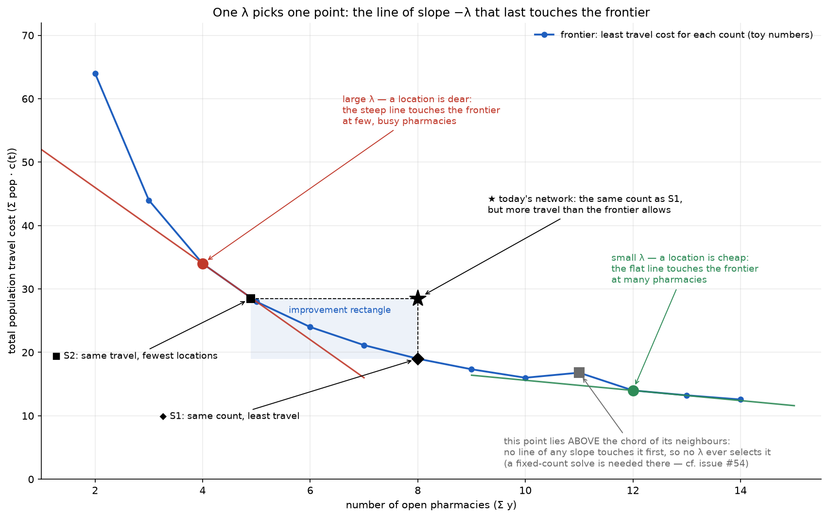
B = (B_x, B_y) is the baseline ★ (today's used cells, today's travel); S1 = (B_x, S1_y) sits straight below it and S2 = (S2_x, B_y) straight left of it, both chord-interpolated between the two frontier points either side of the target (the three S1/S2 definitions: Scenarios S1 S2 S3). Then:
| metric | formula | plain reading | CSV column |
|---|---|---|---|
| corner | C = (S2_x, S1_y) | the rectangle corner opposite the baseline ★ |
corner_* (#48 export only) |
| raw rectangle |
rect_area = (B_x − S2_x)·(B_y − S1_y) |
locations you could close × travel you could save (locations × person-minutes under LINEAR) | rect_area |
| relative rectangle |
rect_rel = (B_x − S2_x)/B_x · (B_y − S1_y)/B_y |
the same two cuts as shares of today's count and travel; in [0, 1] | rect_rel |
| diagonal crossing | where the segment B→C first meets the frontier (diagonal_cross, around line 103) |
cut count and travel by the same share of the largest possible cut in each direction until you hit the frontier: the "balanced improvement" |
cross_x, cross_y
|
| λ at the crossing |
lambda_cross = w(cross_x) · 100 000, w linear in count between the frontier points around the crossing (interp_w_at_x, around line 77) |
the price per location at which the sweep would have chosen roughly the balanced point (its w is interpolated between two solved points, not solved); high means the balanced plan only pays if a location is dear | lambda_cross |
The relative version exists because the raw rectangle "mostly ranks by region size" (comment around lines 124–128; commit 2a6ea08, 20 July 2026); dividing by B_x·B_y also cancels the €100 000 placeholder. The diagonal is what JRC asked for (issue #48, "the requested intersection of the Pareto frontier with the diagonal B→C"); who first proposed the rectangle is not recorded (earliest trace commit e75c73c, 16 July 2026).
Worked toy (reproduced by running metrics_for). Frontier (w, n_open, multi) = (0.1, 100, 40), (0.2, 60, 60), (0.5, 40, 100); B = (80 locations, travel 90).
- S1: between (60, 60) and (100, 40), t = (80 − 60)/40 = 0.5, S1_y = 60 − 0.5·20 = 50 — same count, −44 % travel.
- S2: between (40, 100) and (60, 60), t = (90 − 100)/(60 − 100) = 0.25, S2_x = 40 + 0.25·20 = 45 — same travel, 35 locations surplus.
- C = (45, 50);
rect_area= 35·40 = 1 400;rect_rel= (35/80)·(40/90) = 0.194. - The diagonal B→C meets the segment (40, 100)–(60, 60) at (57.73, 64.55): 22.27 of the 35 closable locations and 25.45 of the 40 avoidable travel units — 63.6 % of each maximal cut. "Balanced" means equal shares of the maximal cuts, not of today's values (here 28 % on both axes only by coincidence).
- λ_cross: w linear in count between (40, w = 0.5) and (60, w = 0.2) at 57.73: 0.5 + 0.886·(0.2 − 0.5) = 0.2341 → €23 409.
The real Netherlands LINEAR row reads the same way (frontier_metrics_interp3.csv: B = (1 615, 60.68 M), S1_y = 48.59 M, S2_x = 1 172.5, rect_rel = 0.2740·0.1993 = 0.0546, crossing (1 382, 54.31 M), λ_cross = €29 154): the balanced plan closes 14 % of today's locations and cuts 10 % of today's travel — 52.7 % of what S2 and S1 respectively show is possible — and is what the optimiser would choose at about €29 000 per location.
When quoting these: (a) the frontier is convex, so a chord runs above it: S1_y, the rectangle and the crossing under-state the saving, never over-state it (file header, lines 13–17). (b) s1_bracketed / s2_bracketed say whether the sweep spanned the target; if not, the value is clamped to the nearest end — at e25416b all 84 rows are bracketed.
doc/frontier_charts.py reads frontier_metrics_<METRIC_SUFFIX>.json and draws, per cost function:
| chart | function | sorted by | x-axis | deck | results page |
|---|---|---|---|---|---|
rank_area_rel_<FN>.png |
rank_bar (around line 93) |
rect_rel |
linear | p73–74 | §4, figures 1–2 |
rank_area_<FN>.png |
rank_bar |
rect_area |
log (raw areas span three and a half orders of magnitude) | p71–72 | — |
rank_lambda_<FN>.png |
rank_bar |
lambda_cross |
linear, € | p69–70 | §4, figure 3 |
pointcloud_<FN>.png |
pointcloud (around line 57) |
— | log–log, locations vs travel | p67–68 | §4, figure 4 |
In the point cloud each area is a ★ at (B_x, B_y) with ◆ S1 straight below, ■ S2 straight left and ● the crossing, joined by thin lines: the vertical stem is the S1 saving, the horizontal stem the S2 saving.
At e25416b the LINEAR rect_rel list reads ITF 0.268, ITG 0.261, ITI 0.129 … FRI 0.016; the λ_cross list ITF €52 807, Denmark €46 380, SE2 €45 168 … Belgium €6 538. The Italian lead is a data artefact: issue #53 showed the ESPON list under-counted southern Italy; on the OECD list ITG and ITF fall to 0.073 and 0.071 (6th and 7th) and SE1, Norway, Lithuania, SE2 and Estonia lead. Never quote a ranking without saying which pharmacy list and which scope rules it was made on (the scope rules #49/#50 moved five areas, #53 moved Italy), and never mix pre- and post-fix rankings.
Bars and stars are coloured to test one hypothesis: does improvement potential follow the pharmacy regulatory regime? Two attributes per country are transcribed by hand in doc/policy_typology.py from slides 11–16 of the JRC typology deck doc/Typology_Countries_to_share.pptx (not tracked in git) into policy_typology.csv (44 rows; each region id inherits its country's attributes): the archetype (T1 rule-of-law-anchored · T2 consensual-pluralist · T3 public-interest majoritarian · T4 segmented-federal; no modelled country is T4) and the formalisation (HIGH / MEDIUM / LOW / VARIES; none is VARIES).
The colour is formalisation (FORM_COLOR: red HIGH, orange MEDIUM, green LOW); the label suffix ·T1 etc. is the archetype — different attributes: Denmark is T2 and red, Belgium T1 and orange. Why colour by formalisation rather than archetype is not recorded beyond "the deck's legend chips" (frontier_charts.py lines 17–18). The finding on the results page: the largest gaps span both HIGH and LOW formalisation — geography dominates regime.
Before 17 July 2026 (commit 559dad9) bars were coloured by a home-made DEGURBA-style urban/rural class from doc/region_typology.jl (Eurostat density bands only, no contiguity step; 14 PU, 28 IN, no PR). Nothing reads region_typology.csv at e25416b, although the header of frontier_charts.py still names it — whether it returns is open.
These describe the observed pharmacy distribution and open the deck (p3–6): the REGIO review asked to describe what exists before what is optimised. Lewis asked for six indicators per country (22 May 2026), originally to set the catchment caps of the A→D ladder, which the observed spread then made unsettable (Alternatives not pursued). GeoDMS computes them (cfg/main/Analyses.dms, container /Analyses/Pharmacies/Descriptives, from line 28, one Arrow row per study area from the item Table — item by item on GeoDMS OD matrix and choice set); make_descriptive_table.bat loops the areas and collect_descriptives.jl gathers doc/pharmacy_descriptives.csv and _nuts1.csv.
The catchment rule. Every inhabited 1 km cell is attached to the pharmacy cell it reaches fastest by road; a location's catchment is the residents of the cells it wins, split equally over the pharmacies in that cell because the data cannot say which one a resident prefers. Road rather than straight-line since 23 June 2026 (commit df77729), because the sweep's baseline assigns by road and a Euclidean descriptive would describe a different network ("Euclidean was wrong"; cell_catchment_euclid is kept for comparison). Caveat: only OD-client cells carry a road-nearest; residents with no pharmacy in their choice set (the 5th-nearest radius capped at 120 min — Scope rules and data gaps) or in an excluded region belong to no catchment, whereas n_residents counts them, so where unreachable residents exist the percentiles and residents_per_pharmacy do not cover the same population (comment around lines 59–62).
| # | indicator (Lewis) | column(s) | definition |
|---|---|---|---|
| 1 | number of pharmacies |
n_pharmacies, n_pharmacy_cells
|
raw points in the area; unique 1 km cells with ≥ 1 pharmacy (a location, the model's unit) |
| 2 | residents per pharmacy |
residents_per_pharmacy = n_residents / n_pharmacies
|
n_residents = Σ population of the 1 km grid over the area |
| 3 | multi-pharmacy cells | n_cells_multi |
cells with cnt > 1 |
| 4 | pharmacies per multi-cell |
avg_pharm_in_multi, max_pharm_in_cell
|
mean cnt over cells with cnt > 1; largest cnt
|
| 5 | per-pharmacy catchment distribution |
pharm_min, pharm_p10 … pharm_p90, pharm_max, pharm_avg
|
percentiles (rth_element) of pharm_catchment
|
| 6 | per-location catchment distribution |
cell_min, cell_p10 … cell_p90, cell_max, cell_avg
|
the same of cell_catchment
|
"Empty" pharmacies. In any clustered country some pharmacy is never the road-nearest for any populated cell (shadowed by a neighbour or, rarely, on a disconnected road fragment); its catchment is 0, so pharm_min is almost always 0 and says nothing. Commit d45019a (23 June 2026) therefore added *_n_empty (how many have catchment 0 — "the redundancy magnitude") and *_min_nz (the smallest non-zero catchment), shown in the deck as #empty and min>0. Netherlands: 1 992 pharmacies in 1 617 cells, 2 empty cells, 4 empty pharmacies. descriptivesSlide in build_deck.mjs (around line 310) renders p3–6; results page §1 has the per-pharmacy country table.
Link to the sweep: a sweep log's baseline cells (base.n_used in baseline_metrics) counts existing-pharmacy cells that are road-nearest for at least one client, i.e. n_pharmacy_cells − cell_n_empty = 1 617 − 2 = 1 615 for the Netherlands. For eight NUTS-1 rows (FRD, FRG, FRH, FRI, FRL, ITH, ITI, SE1) the descriptives slides and the per-area slides' "today" count differ by 1–4 locations; the reason is not recorded — probably the descriptives were regenerated on 3 September 2026 (commit dd2c157) on the post-fix networks while those sweep logs are older.
| what | file → function | notes |
|---|---|---|
| aggregate frontier |
doc/build_charts.py → aggregate_fd, _interp_at, render_aggregate
|
writes agg_data.json; permalink; same rule copied in doc/export_issue48.py → build_aggregate
|
| rectangle, crossing, λ_cross |
doc/frontier_metrics.py → pareto_frontier, interp_y_at_x, interp_x_at_y, interp_w_at_x, diagonal_cross, metrics_for
|
permalink; output frontier_metrics_<suffix>.{json,csv}
|
| ranked lists, point cloud |
doc/frontier_charts.py → rank_bar, pointcloud
|
env METRIC_SUFFIX; reads policy_typology.csv (from doc/policy_typology.py; doc/region_typology.jl is orphaned) |
| aggregate table p59, λ tables p60–61, λ-axis guides |
doc/build_deck.mjs → aggregateSlide, lambdaTableSlide (interp); doc/lambda_axis_chart.py → crossing
|
both log-w |
| descriptives |
cfg/main/Analyses.dms → Pharmacies/Descriptives/Table; make_descriptive_table.bat; collect_descriptives.jl; build_deck.mjs → descriptivesSlide
|
permalink |
| JRC export | doc/export_issue48.py |
issue48_crossings.csv (the metrics above plus € columns, AGGREGATE included), issue48_sweep_results.csv; columns on Log lines and output files
|
Open first: frontier_metrics.py — 194 lines, no matplotlib — and run its functions on the toy rows above.
| name | where | default | what it changes | why you would change it | interactions |
|---|---|---|---|---|---|
METRIC_SUFFIX (env) |
frontier_charts.py around line 23 |
interp1 |
which frontier_metrics_<suffix>.json is charted |
must be interp3 to match the deck; the default silently redraws July |
interp1/2/3 are snapshots, not methods — the argument of frontier_metrics.py (around line 146) only names the output file |
| the €100 000 placeholder |
FACILITY_MIN_COSTS in frontier_metrics.py; FMIN in build_charts.py, lambda_axis_chart.py, build_deck.mjs; FMC in tangent_chart.py
|
100000 | € labels and lambda_cross only |
when a real fixed cost is calibrated (roadmap p63) | five hand copies, not read from settings.jl; rect_rel, the crossing and every ranking are invariant |
SKIP |
frontier_charts.py around line 30 |
{"Poland"} |
areas left out of ranked lists and point cloud | keep disjointness if another country is also swept by parts | mirrors the PL rule in aggregate_fd
|
DECK_ONLY (env) |
build_deck_data.py around line 153 |
all of ORDER
|
restricts deck_data.json to some areas |
a preview deck while sweeps run | the aggregate then sums fewer areas — never publish an aggregate from a partial JSON |
FORM_COLOR, FORM_ORDER
|
frontier_charts.py around lines 19–21 |
HIGH red, MEDIUM orange, LOW green | colour key of bars and stars | to colour by archetype instead | the ·T<n> label suffix stays the archetype |
-
pareto_frontierremoves the wrong point. Its loop (while env and y >= env[-1][1]: env.pop(), around line 43) pops the previous, lower-count point whenever a higher-count row has more travel: on (40, 100), (60, 60), (70, 65) it returns [(40, 100), (70, 65)], losing the better (60, 60); its inline comment says the opposite. Harmless at e25416b (0 pops over all 84 area × function sets), but check before trusting S2_x or the crossing on a noisy area. Not yet filed as an issue. -
Three S1s, two λ rules. S1/S2 come snapped, chord-interpolated or pinned — matrix on Scenarios S1 S2 S3. The aggregate snaps: w = 0.130 (€13 000) on p59 versus S1 λ ≈ €12 984 on the λ-axis chart, which interpolates. And
lambda_crossinterpolates w linearly in count, whereas every other deck λ (build_deck.mjs→interp,lambda_axis_chart.py→crossing) interpolates logarithmically — on the toy €23 409 versus €22 195, 5 % apart for the same point. Whether this is deliberate is not recorded. -
Two x-axes: per-area and aggregate charts plot the fractional
sum_y; metrics, point cloud and λ-axis chart use the integern_open. Per area they differ by at most half a location; in the aggregate, where interpolated per-area values are summed before rounding, by up to about 3 LINEAR / 6 LOGISTIC. -
Stale comments — trust the code. The block comment above
_interp_at(build_charts.pylines 206–207) still says only w present in every area are aggregated; theDescriptivescontainer comment (Analyses.dmsline 26) still says "(Euclidean)";frontier_charts.pylines 1–6 still name DEGURBA;README.md(§ Reporting, around line 99) still says the DEGURBA class colours the ranked lists. - Chord bias is stated, not fixed; the planned cure is the exact fixed-count (p-median) MIP on the roadmap (p63; issue #52's closing comment).
- Open: formalisation vs archetype as colour; whether
region_typology.csvreturns; why_nuts1.csvomits the Polish NUTS-1 rows althoughmake_descriptive_table.batcomputes them —collect_descriptives.jl→nuts1_orderhard-codes NL, FR, IT and SE only, andbuild_deck.mjstitles the slide "FR / IT / SE"; the reason is not recorded.
- The lambda sweep and the Pareto frontier · Scenarios S1 S2 S3 · Deck and charts pipeline · Log lines and output files
- Lambda sweep method (§7) · Pharmacy results September 2026 (§1, §2, §4)
- Scope rules and data gaps · Branches data and environment · Alternatives not pursued · Background theory · Glossary