Repository navigation
The pipeline in plain words
In one sentence: One made-up area ("Toyland": three populated cells, three candidates, two pharmacies today) walked through every stage from the TomTom network to the deck, so that you see what each stage consumes, decides and writes before opening the detailed pages.
Where this sits: The map of the whole chain — GeoDMS → Arrow → Julia baseline → LP → λ-sweep → rounding → S1/S2 → outputs → deck; each stage ends with the page that owns it. Maarten's formal version: Pharmacy service access, Lambda sweep method; what a checkout can reproduce: Branches data and environment.
As of September 2026 (commit e25416b); terms in italics are in the Glossary.
Three engines hand each other files on disk. GeoDMS costs seconds to minutes per area, the Julia sweep minutes to hours; doc/ post-processes the logs.
flowchart TD
TT[TomTom streets, population grid, pharmacy points] --> G[GeoDMS cfg/main.dms<br/>STUDY_AREA = area, once per side]
G -->|ExistingPharmacies/<area>_od,_i,_j.arrow| B[Julia baseline_metrics<br/>today's network scored by the model]
G -->|NewPharmacies/<area>_od,_i,_j.arrow| LP[Julia build_lp_warmstart<br/>one LP per area]
B --> SW[lambda_sweep_simplex.jl<br/>solve_at_w! per grid point, round, pin S1 and S2]
LP --> SW
SW -->|logs/sweep_<area>_<FUNC>.log| P[doc/build_deck_data.py<br/>deck_data.json]
SW -->|lambda_sweep/<FUNC>/w=…, S1, S2/<br/>assignment.arrow, traveltime.arrow| M[GeoDMS ReadSweepResults_T<br/>maps of S1 and S2]
SW -->|S1, S2 assignment.arrow| X[export_s1s2_locations.jl<br/><area>_s1_linear_open.arrow for JRC]
P --> C[build_charts.py, frontier_metrics.py, build_deck.mjs, merge_deck.ps1]
C --> D[doc/lambda_sweep5.pptx]
Three inhabited 1 km² cells, two pharmacies today; travel cost LINEAR, c(t) = t in minutes (LOGISTIC: Travel cost functions).
| cell | residents | pharmacy today? | candidate? | why a candidate |
|---|---|---|---|---|
| A (town) | 600 | no | yes | ≥ 50 residents |
| B (village) | 300 | yes | yes | holds a pharmacy |
| C (hamlet) | 60 | yes | yes | holds a pharmacy |
Road times in minutes: A–B 6; B–C 115, so A–C is 121 — beyond the 120-minute cut-off, and the model never sees that pair. A cell to itself is 1 second (MinTime := 1[s_f]). A candidate needs at least 50 residents or a pharmacy today (MinPopSizeForPharmacyLocation := 50, cfg/main/ModelParameters.dms; NewPharmacyLocations, cfg/main/SourceData/Locations.dms); why 50 and what it cost in Luxembourg: GeoDMS OD matrix and choice set.
For one study area (STUDY_AREA) GeoDMS builds the road network, runs impedance_matrix_od64 from each client cell to the candidates in its choice set — every candidate within the road time to the client's 5th-nearest existing pharmacy, capped at 120 min; 71–86 per client on average (deck p5, commit 4267fe0) — and exports <area>_od.arrow (one row per client–candidate pair), <area>_i.arrow (clients) and <area>_j.arrow (candidates). It runs twice: the Existing side (ProjName = 'ExistingPharmacies', today's pharmacy cells) only scores today's network; the New side ('NewPharmacies', all candidates) is what the optimiser works on. Why 5 and 120 is not recorded; the radius is today's and can bind once cells close (Scope rules and data gaps).
Toyland's New-side files. _i.arrow rows 0–2 are A, B, C and _j.arrow rows 0–2 their cells; the OD uses those ids, and t_ij is seconds:
| client_rel | facility_rel | t_ij (s) |
|---|---|---|
| 0 | 0 | 1 |
| 0 | 1 | 360 |
| 1 | 0 | 360 |
| 1 | 1 | 1 |
| 1 | 2 | 6900 |
| 2 | 1 | 6900 |
| 2 | 2 | 1 |
The Existing side has its own _j.arrow (0 = B's cell, 1 = C's) and a five-row OD; ids are local per file, so Julia matches baseline cells to candidates by rounded (x, y) (load_from, around line 95).
Read next: GeoDMS OD matrix and choice set (the directives, the exports); Scope rules and data gaps.
baseline_metrics (lambda_sweep_simplex.jl, around line 167) sends every client to its nearest existing pharmacy, sums c(t) × residents, and counts the pharmacy cells that are somebody's nearest — today's count, in cells. A client absent from the Existing OD pays BIG = c(120 min), 120 under LINEAR and 1.0 under LOGISTIC (big_cost(); why: Travel cost functions), so the baseline is coverage-consistent with what the optimiser builds.
Toyland. A → B (6 min), B → B (1 s), C → C (1 s); nobody is unreachable.
- travel cost = 600·6 + 300·(1/60) + 60·(1/60) = 3 600 + 5 + 1 = 3 606 person-minutes
- cells used = 2; mean travel time = 3 606 / 960 residents = 3.756 min
This is the log's first block; files land under ExistingPharmacies\Toyland\lambda_sweep\LINEAR\baseline\. The baseline ★ = (2 cells, 3 606) is what the scenarios are measured against: S1 is the frontier point at today's count, S2 the point at today's travel, S3 the whole frontier (Scenarios S1 S2 S3).
build_lp_warmstart (lp_run.jl, around line 397) builds the facility-location LP once per area on the New side — y_j per candidate ("how open is cell j", 0 to 1) and x_k per OD row ("what share of that client is served there"), solved exactly and fast by HiGHS via JuMP. solve_at_w!(state, w) (around line 460) prices every y_j at λ = w × FACILITY_MIN_COSTS = w × €100 000 and minimises
travel cost of the served shares  +  BIG × unserved shares  +  λ × Σ_j y_j
subject to   Σ_k x_k ≤ 1 per client  (soft coverage)   and   x_k ≤ y_j  (only use an open cell)
In words: pay every resident's travel, BIG per unserved resident and λ per open location; find the cheapest mix. w is the dimensionless knob, λ the same knob in placeholder euros (The lambda sweep and the Pareto frontier). Why fractions rather than yes/no, and why ≤ 1 (soft coverage: a client may be abandoned when serving it costs more than BIG): The facility location model explained.
Toyland at w = 0.02 (λ = €2 000). Total = travel + λ × count ({C} and {} are far worse):
| open cells | travel (person-min) | + λ × count | total |
|---|---|---|---|
| A, B, C | 16 | 6 000 | 6 016 |
| A, C | 10 + 300 × 6 + 1 = 1 811 | 4 000 | 5 811 |
| B, C (today) | 3 606 | 4 000 | 7 606 |
| A, B | 10 + 5 + 60 × 115 = 6 915 | 4 000 | 10 915 |
| A only | 10 + 1 800 + 60 × 120 (C unserved) = 9 010 | 2 000 | 11 010 |
The LP returns y = (1, 0, 1): open A, close B, keep C — the village pharmacy moves to the town. sum_y = 2.0, frac_y = 0, travel_relax = 1 811 (the LP's own travel, the lower bound); in real areas a few dozen y_j are fractional.
Read next: The facility location model explained; Travel cost functions; Code walkthrough lp_run.
The rest of solve_at_w! turns the fractions into a network of exactly p = round(sum_y) open cells, three ways — top-p, greedy and multistart (the default ROUNDING) — and travel_of scores each set: every client to its nearest open cell, BIG where none is in reach (stranded). The seeds, the swap polish, why multistart is the default and the certified gap between it and the LP: From LP fractions to real pharmacies.
Toyland at w = 0.02. p = 2. Top-p = {A, C}; greedy and multistart also give {A, C}. All score 1 811 person-minutes, nobody stranded, so cost_c = 1 811 — the number S2 is measured on; mean travel time 1 811 / 960 = 1.8865 min.
analyze_country repeats Stages 3–4 for a fixed grid of prices — w = 1, 2, 5 per decade from 1e-4 to 5.0 for LINEAR (15 points), to 0.5 for LOGISTIC (12) — and HiGHS warm-starts each solve from the previous basis, so a further point costs a small fraction of the first (The lambda sweep and the Pareto frontier). Each solved point is one point of the Pareto frontier, the least travel achievable for that count.
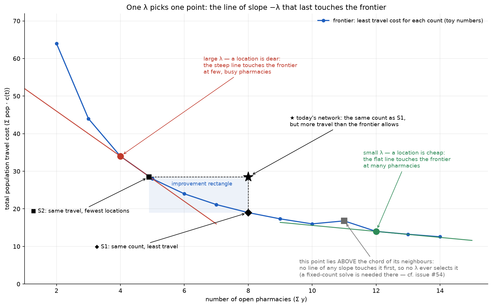
Pinning S1 and S2. The S1 bracket closes when sum_y falls through the baseline count between grid points, the S2 bracket when cost_c rises through the baseline travel; the driver then bisects the bracket at the geometric midpoint sqrt(lo·hi) until the residual is within REFINE_TOL (0.2 % of the target; at least one whole cell for S1) or eight solves, and restores the basis. Why bisect the moment a bracket closes, and refine-only mode: Scenarios S1 S2 S3.
Toyland's sweep (rows beyond w = 0.1 omitted):
| w | sum_y | travel_multi | n-cells | what happened |
|---|---|---|---|---|
| 1e-4 … 0.01 | 3.0 | 16 | +1 | open everything |
| 0.02 | 2.0 | 1 811 | 0 | S1 bracket closes (sum_y 3 → 2 through 2) |
| 0.014142 | 3.0 | 16 | +1 | S1 bisection: residual 1 = tolerance; S1 pinned at w=0.02
|
| 0.05 | 2.0 | 1 811 | 0 | still {A, C} |
| 0.1 | 1.0 | 9 010 | −1 | C's cell costs λ = 10 000, saves only 60 × (120 − 1/60) ≈ 7 199: stranded; S2 bracket closes |
| 0.070711 … 0.084090 | 2 or 1 | 1 811 or 9 010 | 0 or −1 | eight S2 bisections round the jump at λ = 7 199; none within ±7.2 |
The log prints S2 pinned at w=0.05: cost_c=1811.0 (target 3606.0) — 50 % off, and "pinned" is printed regardless: a three-step staircase has no point at today's travel; on a real area the halving soon fits the tolerance. Always read the residual. closest() then picks the exported rows, the snapped row nearest the target; in Toyland both S1 and S2 snap to w = 0.02 (issue #52's "S1 = S2" in miniature).
Read next: The lambda sweep and the Pareto frontier; Scenarios S1 S2 S3.
The log. One text file per area and function, logs\sweep_<area>_<FUNC>.log (a refine-only rerun, SWEEP_STOP_AFTER_REFINE=1, writes logs\refine_<area>_<FUNC>.log); print_sweep_row prints one line per solved point — Toyland's w = 0.02 row:
w           λ (€)         sum_y       travel_relax    travel_topp     travel_greedy   travel_multi    n_open    fac_€         mean_t    frac_y    n-cells
0.02        2000.0        2.0         1811.0          1811.0          1811.0          1811.0          2         200000.0      1.8865    0         0
The story's columns: sum_y (LP count), travel_relax (lower bound), travel_multi (the rounded network — the curve the deck draws), n-cells (distance from today's count; 0 = S1). Every column with its unit: Log lines and output files.
The Arrow outputs. Per rounded point, on the New side: <area>\lambda_sweep\<FUNC>\w=<w>\assignment.arrow (id, open 0/1) and traveltime.arrow (id, t_ij in minutes; a stranded client has no row); the snapped S1 and S2 are copied to S1 and S2 folders. Toyland at w = 0.02: assignment.arrow = (0,1), (1,0), (2,1). GeoDMS reads them via ReadSweepResults_T (cfg/main/Analyses.dms, around line 219); export_s1s2_locations.jl joins S1/S2/assignment.arrow to _j.arrow into <area>_s1_linear_open.arrow for JRC (issue #45).
Read next: Log lines and output files; Running a sweep end to end.
doc/build_deck_data.py parses the sweep and refine_ logs for every area in ORDER into doc/deck_data.json — baseline, frontier rows, snapped S1/S2; build_charts.py draws the charts, frontier_metrics.py the improvement rectangle, build_deck.mjs and merge_deck.ps1 assemble doc/lambda_sweep5.pptx.
Which S1/S2 is which. Deck tables and chart markers are chord-interpolated between the two frontier points bracketing the target (build_deck.mjs → interp; build_charts.py → interp_s1_s2); exported files use the snapped, pinned rows (the matrix of the three definitions: Scenarios S1 S2 S3). The improvement rectangle between star and frontier and the balanced improvement on its diagonal rank the areas (Metrics aggregation and ranking).
Toyland on the slide. Pareto envelope of (n_open, multi): (1, 9 010), (2, 1 811), (3, 16). S1 by chord at count 2: 1 811 → −49.8 % travel. S2: the chord from (1, 9 010) to (2, 1 811) passes 3 606 at count = 1 + (3 606 − 9 010)/(1 811 − 9 010) = 1.751 → −12.5 % locations (a fraction; the exported file holds two). Relative rectangle = 0.125 × 0.498 = 0.062.
Read next: Deck and charts pipeline; Metrics aggregation and ranking.
| stage | open first, then |
|---|---|
| 1 GeoDMS |
cfg/main/Analyses.dms → Allocate_T/Allocation (impedance_matrix_od64, around line 277); cfg/main/SourceData/Locations.dms → NewPharmacyLocations; cfg/main/ModelParameters.dms
|
| 2 baseline |
lambda_sweep_simplex.jl → load_from, baseline_metrics; settings.jl → big_cost
|
| 3 LP |
lp_run.jl → build_lp_warmstart, solve_at_w!; settings.jl → c(t), FACILITY_MIN_COSTS
|
| 4 rounding |
lp_run.jl → multistart_round, greedy_round, swap_round!, travel_of; settings.jl → ROUNDING
|
| 5 sweep |
lambda_sweep_simplex.jl → analyze_country (loop around line 387), bisect!, refine_if_closed!; lp_run.jl → resolve_for_basis!
|
| 6 outputs |
lambda_sweep_simplex.jl → print_sweep_row, write_scenario_arrows, closest; cfg/main/Analyses.dms → ReadSweepResults_T; export_s1s2_locations.jl
|
| 7 deck |
doc/build_deck_data.py → parse; doc/build_deck.mjs → interp; doc/build_charts.py → interp_s1_s2; doc/frontier_metrics.py
|
Permalinks pinned to the documented commit: lp_run.jl#L397, lambda_sweep_simplex.jl#L167, lambda_sweep_simplex.jl#L387, Analyses.dms#L277.
-
Units change at the border:
t_ijis seconds in_od.arrow, minutes in Julia; costs are person-minutes (LINEAR) or dimensionless (LOGISTIC); counts are cells — the units table is on Log lines and output files. -
HiGHS's own objective is negative: it drops the constant
BIG × population(Toyland: 5 811 − 115 200 = −109 389); readtravel_relax(The facility location model explained). -
mean_tis not coverage-consistent: sweep rows count stranded clients at 0 minutes (lp_run.jlaround line 551), the baseline at 120 — Toyland at w = 0.1 reports 1.8854 while stranding C; comparecost_c(Log lines and output files). -
The issue-#52 "climb" commits are not on GitHub as of 15 September 2026 (Branches data and environment); the
S1/S2folders are overwritten by every run.
- Home · Branches data and environment · FAQ · Glossary
- GeoDMS OD matrix and choice set · Scope rules and data gaps · The facility location model explained · Travel cost functions · From LP fractions to real pharmacies · The lambda sweep and the Pareto frontier · Scenarios S1 S2 S3 · Metrics aggregation and ranking
- Log lines and output files · Running a sweep end to end · Deck and charts pipeline