Repository navigation
The lambda sweep and the Pareto frontier
In one sentence: solving the same facility-location LP (the linear-programming relaxation of the "where to open pharmacies" problem; Glossary) at a rising price per location traces the trade-off between "how many pharmacies" and "how far people travel"; this page explains why that works, what the curve cannot show, and how to read the two charts drawn from it.
Where this sits: GeoDMS exports the OD matrix and the two facility sides (GeoDMS OD matrix and choice set) → Julia builds one LP per area (The facility location model explained) → the sweep over λ (this page) → each point is rounded to real pharmacies (From LP fractions to real pharmacies) → S1/S2 are read off the curve (Scenarios S1 S2 S3) → aggregation and ranking (Metrics aggregation and ranking) → the deck (Deck and charts pipeline). Maarten's compact formal statement is Lambda sweep method.
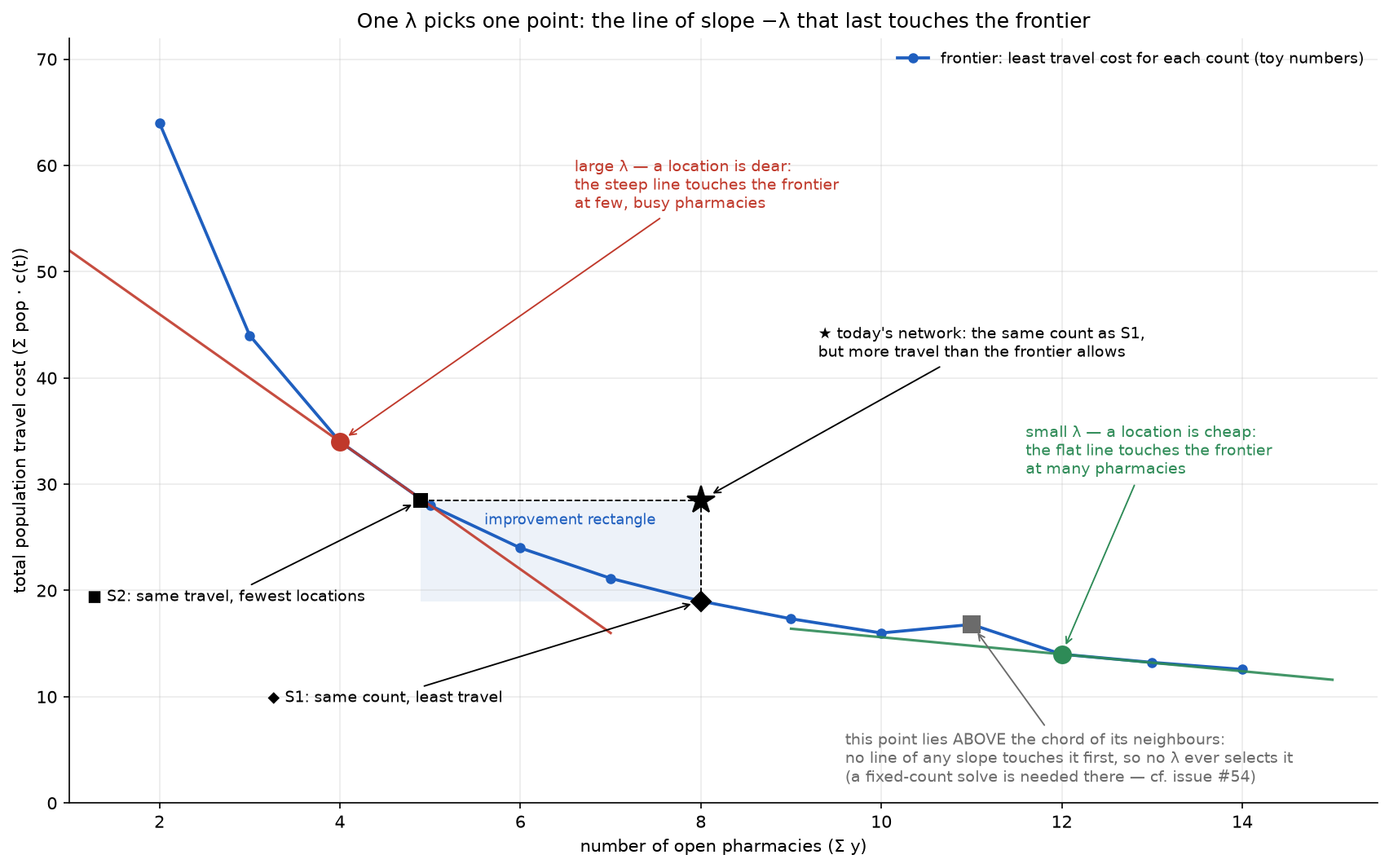
Put every achievable network in a plane: x = number of open pharmacies, y = total population travel cost Σ pop · c(t), where c(t) is the cost of one trip of t minutes (Travel cost functions). The LP minimises travel + λ · count; λ (lambda; Glossary) is the price of keeping one pharmacy cell open, and the only thing that changes between two points of a sweep.
Travel + λ · count is constant along a straight line of slope −λ. Minimising it means sliding that line down until it last touches the cloud of achievable points; the touching point is the optimum for this λ. A steep line (large λ, a location is dear) touches at few, busy pharmacies; a flat line at many. A sweep is nothing more than: change the slope, find the new touching point.
A worked example: three clients of 100 residents, three candidate cells, LINEAR cost, minutes A→1 = 5, A→2 = 20, B→1 = 15, B→2 = 10, B→3 = 30, C→2 = 25, C→3 = 5 (other pairs outside the choice set, the candidates a client may use; Glossary). The best network at each count — the other subsets lose ({2, 3} costs 3 500, {1, 2} 4 000, {1} and {3} strand a client) — is: all three open, travel 100·(5+10+5) = 2 000 person-minutes; {1, 3}, 2 500; {2} alone, 5 500; nothing open, everyone stranded at BIG = 120 min, 36 000. Add λ × count:
| λ (€) | all three | {1, 3} | {2} | nothing | picked |
|---|---|---|---|---|---|
| 100 | 2 300 | 2 700 | 5 600 | 36 000 | all three |
| 1 000 | 5 000 | 4 500 | 6 500 | 36 000 | {1, 3} |
| 10 000 | 32 000 | 22 500 | 15 500 | 36 000 | {2} |
The count falls as λ rises and jumps at the break-even prices, where two options cost the same: all three vs {1, 3} gives 2 000 + 3λ = 2 500 + 2λ, so λ = 500; likewise λ = 3 000 and λ = 30 500. The LP relaxation follows the same logic with a fractional count, sum_y (columns table below; Glossary).
Three things follow, and the code relies on each:
-
The count never rises when λ rises — a set with more locations that was optimal at a higher price would have been optimal at the lower one too. This is why the S1 bisection (Scenarios S1 S2 S3) searches on
sum_y. - The lower-left envelope of all touching points is the Pareto frontier (Glossary): no achievable network has both fewer pharmacies and less travel than a frontier point. The frontier depends on the geography and the cost function only; λ just says which point a decision-maker with that price would choose. Hence the deck reports gains in native units — cells, person-minutes — and in € only as a secondary label that depends on the placeholder price below.
- Today's network is a point in the same plane — the baseline ★, scored by the same rule as every LP point — above the frontier. S1 is the frontier point with today's count, S2 the one with today's travel; both are defined by count and travel, never by a λ (Scenarios S1 S2 S3).
The knob you set is w, dimensionless; λ is w times a placeholder price: λ = w * FACILITY_MIN_COSTS (lp_run.jl → solve_at_w!, around line 464) with FACILITY_MIN_COSTS = 100000 in settings.jl (around line 17, env-overridable). So w = 0.2 means λ = €20 000 per location; the log prints both.
Why the € is a placeholder. The number is inherited, not estimated: the school-era model priced a school at €99 699 fixed plus €3 277.5 per pupil (Jacobs-Crisioni et al. 2023, doc/topics.md; issue #38, Maarten: keep linear facility costs). When the settings became env-driven (40a3d55, 24 May 2026) these were rounded to 100 000 and 3 333 as placeholders for pharmacies. Nobody has calibrated a pharmacy value; the deck labels it a placeholder (b3c634b, 4 September 2026; Decision log). Why it was never re-estimated is not recorded.
It is harmless because the LP only ever sees λ and the frontier is a property of the geography and c(t) alone. A different constant leaves the curve, the star, S1 and S2, the native-unit gains and the ranking of areas unchanged; it changes the € printed next to them (the λ (€) and fac_€ log columns, the deck's λ tables, the "λ at the crossing" metric in Metrics aggregation and ranking) and, because the grid is fixed in w, which λ the grid points visit — the solved points slide along the same curve. Before re-running with a calibrated value read the Knobs row: the constant is copied five times in doc/.
A sliding straight line can only touch the convex hull of the cloud (the shape of a rubber band stretched around all the points; Glossary). If at some count p the best network sits above the chord (straight segment) joining the best networks at p − 1 and p + 1 — a concave dent — the line touches a neighbour first whatever its slope, and no λ produces exactly p locations: the count jumps over p.
Example (three clients, four candidates; travel in minutes for one resident each, λ in the same units, not €):
        cand0  cand1  cand2  cand3
   A     10      0     20     20
   B     10     20      0     20
   C     10     20     20      0
Best travel with 1, 2, 3 sites is 30 (cand0), 20 ({0, 1}), 0 ({1, 2, 3}). The chord from (1, 30) to (3, 0) passes through (2, 15), below 20. Two sites beat one site only while a site costs at most 10 (20 + 2λ ≤ 30 + λ), and beat three sites only once a site costs at least 20 (20 + 2λ ≤ 3λ) — no price does both. The count goes 3 → 1 at λ = 15, and a bisection aimed at "today's count = 2" would bounce between the endpoints.
Two consequences:
- The sweep never asks for exactly p pharmacies; it prices them, so it finds only the counts where a straight line can rest on the curve of "least travel for p sites" — its sagging lower outline (in OR terms a Lagrangian relaxation of the p-median problem, reaching only the lower convex envelope of its value function; Background theory, Glossary). If today's count sits in a dent, S1 can only be chord-interpolated between the bracketing points — conservative, because a chord lies above a convex curve (Scenarios S1 S2 S3) — or solved with a fixed-count model, a roadmap item (
doc/todo.mditem 5). In practice dents are shallow: with tens of thousands of candidates the curve is nearly smooth, and S1 was pinned within 1 % (or one facility) in 87 of 88 sweeps (issue #52). - A visible dent in the plotted LP bound means two problems were mixed, because one LP's curve must be convex. Issue #54 (FRI LINEAR): the grey lower bound had bumps because its rows alternated between the July sweep (a 3× candidate subsample) and the September refine-only points (full candidate set), so λ did not fall steadily as the count rose — Maarten's tell. Fix: re-sweep FRI in full. Sixteen more areas mix a July sweep with a rebuilt OD (kinks ≤ 1.5 %; per-area provenance in Branches data and environment).
The sweep solves the LP at a fixed list of w (lambda_sweep_simplex.jl around lines 304–312):
- 1-2-5 per decade from 1e-4 upwards: 0.0001, 0.0002, 0.0005, 0.001, … The grid is geometric (equal ratios, not equal steps) because the interesting λ spans five decades and, per the comment around line 318, a ×2–2.5 step moves the count by a roughly constant ~30 % wherever it sits; that is also why the bisection halves the bracket in log w and the charts interpolate log-in-w. Why 1-2-5 rather than, say, √10 steps is not recorded.
-
Per-function top
w_max:SWEEP_WMAXif set, else 0.5 for LOGISTIC and 5.0 for LINEAR — LINEAR 15 points (1e-4 … 5), LOGISTIC 12 (1e-4 … 0.5). LOGISTIC needs a lower range because its c(t) spans 0.08–1 against 0–120 for LINEAR, so the aggregate's useful λ-range is only €10–€2 000 (w 1e-4 … 0.02) against €10–€50 000 under LINEAR — the λ-compression problem, the "degeneracy" of deck p64 (Travel cost functions). - Common to every area, because the aggregate frontier sums per-area rows at equal λ; an area that stops early truncates the range every area covers (Metrics aggregation and ranking).
-
SWEEP_MULTSreplaces the multipliers, e.g.1,1.5,2,3,5,7— the "Round-2 densification" used for the Netherlands rows indeck_data.json, halving the gap in 0.2–0.5 where the crossings cluster. The decade loop runs tod_hi = max(0, ceil(log10 w_max)), soSWEEP_WMAX=20adds 10 and 20 to the grid rather than stopping at 5.
History (dated rows in Decision log). The first driver (011cafb, May 2026) stopped early per area, truncating the aggregate; 206923c (6 July) fixed a common grid to 5.0 plus a per-area upward extension until S1 was bracketed. The top of that grid proved intractable under hard coverage (Netherlands LINEAR at w = 5.0 took 16.7 h): 86476bf (7 July) switched to IPM + crossover from w = 0.5 upward and added LP_TIME_LIMIT at 4 h, so that a pathological point becomes a skipped point rather than a stall; f93aea1 (9 July) removed the extension, capped w_max per function at 1.0 LINEAR / 0.02 LOGISTIC, made every solve IPM + crossover and lowered the limit to 3600 s; acd59a6 the same day went back to warm-start simplex for LINEAR after the Netherlands timed out on every point from w = 0.005. Soft coverage (agreed 10 July, committed 4ec47a9 16 July; The facility location model explained) made high-λ solves cheap, and w_max went back up to today's 5.0 / 0.5, high enough that every area brackets both scenarios. Several texts still describe the extension (Pitfalls). If S1 is not bracketed at w_max the driver only prints a hint to raise SWEEP_WMAX (around line 420); under soft coverage sum_y keeps falling as λ rises, so a higher w_max always brackets eventually.
build_lp_warmstart builds the LP once per area; solve_at_w! sets only the objective coefficients of the y variables to λ (around lines 466–469) and calls optimize! on the same HiGHS instance. The x side of the objective never depends on λ — BIG and c(t) do not — so nothing is rebuilt; the "constant drops out" trick that makes this possible, and why HiGHS's printed objective is therefore negative, is on The facility location model explained.
Why the next solve is cheap: the simplex method (Glossary) sits at a corner of the feasible region, described by a basis (the variables allowed to be non-zero). The constraints did not change, so the old corner is still feasible; only the prices did, so it is merely no longer optimal. Dual simplex repairs exactly that, and for a small change in λ only a few reduced costs (the change in objective per unit of a variable currently at zero) change sign, so few pivots (steps to a neighbouring corner) are needed. HiGHS picks dual simplex for these re-solves (its default; confirmed in the May 2026 hard-coverage logs, unverified since — Pitfalls) and detects the reusable basis ("Solving LP with useful basis so presolve not used"): in the old Netherlands log the cold solve took 45 876 iterations, the next point 1 369.
When it fails: a large absolute step in λ (at the top of the grid a 1-2-5 step moves every y-price by 10⁵–10⁶) flips thousands of reduced costs at once, the old basis is far from the new optimum and the LP is highly degenerate (many corners share one objective value, so pivots make no progress) — the "cliff" that cost 16.7 h under hard coverage and now bites only the largest LINEAR areas. The residual danger is a timeout: LP_TIME_LIMIT (lp_run.jl around line 439) turns a pathological point into a skipped point, but HiGHS is left on an aborted basis and later points warm-start from it and tend to time out too (issue #52). Hence the driver bisects S1/S2 the moment their bracket closes, restores the basis afterwards (resolve_for_basis!) and stops the tail at the first timeout (SWEEP_STOP_AFTER_TAIL_FAIL): reasoning on Scenarios S1 S2 S3, code on Code walkthrough lambda_sweep_simplex.
IPM instead (SOLVER=ipm, around line 483). An interior-point method (Glossary) ignores any basis and costs about the same per solve whether the previous point was near or far; crossover then pushes its interior answer to a corner so that sum_y, frac_y and the rounding see a clean solution. Right tool for a single far solve on a giant LINEAR area (Belgium/FRI, 2b60d00); wrong tool for a chain of near steps (the IPM days of July, History above). It fails outright on soft-coverage LOGISTIC (every ITG point OTHER_ERROR; the comment around lines 471–482 blames the coefficient range, x-coefficients down to −7.5e-5 · pop next to λ up to 5 · 10⁴).
Each solved point prints one log row (Log lines and output files has every column, with units); four carry the sweep's meaning:
| column | what it is | how to read it |
|---|---|---|
sum_y |
Σ_j y*_j, the LP's fractional facility count (around line 501) | the x-coordinate of the LP point; falls monotonically with w; S1 is where it crosses today's cell count |
frac_y |
number of candidates with 1e-6 < y*_j < 1 − 1e-6 (around lines 499–500) | how non-integral the relaxation is; tens out of thousands means the LP is almost a real network. It grows where the geography resists a clean covering and at high λ, where the LP splits the last facilities (Netherlands LOGISTIC: 612 fractional at w = 0.02 for 403 open; LINEAR: 530 at w = 1.5 for 406 open), though not monotonically (Netherlands LOGISTIC: 36 at w = 0.5) |
travel_relax |
served travel + BIG × each client's unserved share (lines 502–513) | the coverage-honest lower bound on travel at this λ (stranded clients charged BIG, the rule the baseline and the rounding also use); not HiGHS's printed objective (Pitfalls) |
travel_multi (= cost_c) |
travel of the multistart rounding, stranded clients at BIG (From LP fractions to real pharmacies) | the upper bound; the curve the deck plots as "the frontier" |
sum_x and frac_x are the same quantities in logs before 24 July 2026 (4cee238 swapped x and y to the p-median convention; The facility location model explained). Fractional sum_y is information, not noise — Maarten's ½-½-½ example on Lambda sweep method has the LP strictly beating every integer network.
Together the two curves sandwich the best real network at price λ: travel_relax + λ·sum_y ≤ integer optimum ≤ travel_multi + λ·n_open. This is a statement about travel + λ · count together, not about the travel at a given count; what the reported gap does and does not certify is on From LP fractions to real pharmacies.
Axis-by-axis detail (element → field → script) is in Deck and charts pipeline; here is what the two charts mean.
The frontier chart (doc/build_charts.py → render; one per area and function, e.g. images/Netherlands_LINEAR.png):
- x =
sum_y, the fractional LP count — the one chart that does not usen_open; why is not recorded (the difference is under one facility, though the deck table interpolates the S1 λ onsum_yand the S1 gain onn_open,build_deck.mjsaround lines 518 and 547). Left y = total travel: person-minutes under LINEAR (axis from zero), dimensionless under LOGISTIC, whose axis is stretched to the data (non-zero origin) so the tiny gap between the bounds is visible. -
Solid blue =
travel_multi, the upper bound; dashed grey =travel_relax, the lower bound, drawn on top so it stays visible where the two coincide. Blue-under-grey means the relaxation is essentially integral; where they separate (the low-count end) the rounding is losing something. Amber dashed, right axis = log₁₀ λ in €, the chart's only trace of λ. - ★ = today's network; ◆ S1 (blue) on the blue curve directly below it; ■ S2 (purple) where the blue curve crosses today's travel. Charts and deck tables interpolate between rows; the exported location files use the nearest solved row, which before #52 could be a grid step away (Netherlands: w = 0.3 with 1 334 open) — Scenarios S1 S2 S3 explains both readings.
The λ-axis chart (doc/lambda_axis_chart.py; deck p65–66; images/lambda_axis_AGGREGATE.png, images/lambda_axis_Netherlands.png) reads the same sweep along λ (x, log scale; LINEAR and LOGISTIC panels), because the frontier chart hides where along the sweep the bounds open up and how fast the count collapses. Left axis: the two travel bounds and today's travel; right axis (log): n_open, sum_y and today's count. Vertical guides mark the S1 and S2 crossings, interpolated log-in-w as the deck's λ tables do; since 1ed57f2 each level line says what defines it and the S1 crossing carries λ · N, the facility bill at that price.
- Reading, on the aggregate LINEAR panel (41 areas): the count is flat at "open everything" below λ ≈ €100, then falls over two decades; the travel bounds lie on top of each other until just past S2 (€22.6 k interpolated on the λ-axis chart; the aggregate table on Pharmacy results September 2026 snaps to the nearest union row, w = 0.227, i.e. €22 700). On the Netherlands LINEAR panel they coincide up to ~€50 000, beyond its S2 at €34 329, so its S1 and S2 sit where lower and upper bound agree. Under LOGISTIC everything happens between €10 and €2 000.
- The wiki's
images/lambda_axis_*.pngare an older render (linear count axis, no level labels); the current render is committed indoc/img/and embedded inREADME.md. Only the git-ignoreddoc/charts/folder, where the scripts write, lives on the machine that ran them.
| what | where |
|---|---|
λ from w; y-coefficients rewritten; solver, crossover, time limit; sum_y, frac_y, travel_relax
|
lp_run.jl → solve_at_w! — permalink
|
LP_TIME_LIMIT and the solver-history comment |
lp_run.jl around lines 432–439 |
| basis restore after a bisection detour |
lp_run.jl → resolve_for_basis!, around line 445 |
w_max, mults, ws_common, and why the grid is common and per function |
lambda_sweep_simplex.jl around lines 293–312 — permalink
|
| grid loop with interleaved bisection and tail stop |
lambda_sweep_simplex.jl around lines 385–415 |
| the log row |
lambda_sweep_simplex.jl → print_sweep_row, around line 221 |
FACILITY_MIN_COSTS, FACILITY_CLIENT_COSTS, facility_cost
|
settings.jl around lines 17–18 and 99 |
| frontier chart, λ-axis chart, tangent slide |
doc/build_charts.py → render; doc/lambda_axis_chart.py → panel, crossing; doc/tangent_chart.py
|
Open solve_at_w! first: everything on this page is one of its inputs or outputs. Function-by-function detail: Code walkthrough lp_run, Code walkthrough lambda_sweep_simplex.
| name | default | what it changes | why you would change it | interactions |
|---|---|---|---|---|
FACILITY_MIN_COSTS |
100000 | λ = w · this; every € label | only if a real location cost is agreed | the deck scripts do not read settings.jl: 100 000 is hard-coded five times in doc/ (FMIN in build_charts.py, lambda_axis_chart.py, build_deck.mjs; FACILITY_MIN_COSTS in frontier_metrics.py; FMC in tangent_chart.py) and all five must follow; frontier and S1/S2 do not move, but the fixed w-grid then samples different λ |
SWEEP_WMAX |
5.0 LINEAR / 0.5 LOGISTIC | top of the grid | raise when the driver says S1 is not bracketed; lower to skip an expensive tail | must be equal across every area in one aggregate |
SWEEP_MULTS |
1,2,5 |
per-decade multipliers | densify where crossings cluster (1,1.5,2,3,5,7) |
the post-loop "fine sweep" (a retry of grid multipliers between the S1 and S2 brackets that failed earlier; Code walkthrough lambda_sweep_simplex) uses the same list, so adds nothing new |
SOLVER |
simplex |
ipm = interior point + crossover |
a giant LINEAR area stuck on the simplex cliff | never for LOGISTIC (OTHER_ERROR); every IPM point pays full price, no warm start |
LP_TIME_LIMIT |
3600 s | HiGHS time_limit per solve |
Poland-size LPs (issue #52 mentions 4 h) | a timeout poisons the warm start of later points |
TRAVEL_FUNC |
QUADRATIC |
c(t), BIG, w_max default, output folder |
always set LINEAR or LOGISTIC — the default sweeps a function nobody reports | Travel cost functions |
The bisection knobs (REFINE_TOL, REFINE_ITERS, SWEEP_STOP_AFTER_REFINE, SWEEP_STOP_AFTER_TAIL_FAIL) belong to Scenarios S1 S2 S3.
-
Stale text about the upward extension in Lambda sweep method §2,
README.mdline 133,doc/todo.mditem 4 and the header ofrun_resweep_batch.ps1; the grid has been fixed tow_maxsincef93aea1. - A non-convex plotted lower bound is a provenance error, not a feature (issue #54): every row of an area's frontier must come from one sweep on one OD and one candidate set.
-
The HiGHS objective value in the log is not the travel cost: it equals
travel_relax − BIG·Σpop + λ·sum_y(constant dropped, facility bill included); readtravel_relax. -
fac_€issum_y× 100 000 whilen_openis round(sum_y) — the two columns disagree by up to €50 000. -
FACILITY_CLIENT_COSTS = 3333is dead code: onlyfacility_cost(q)(settings.jlaround line 99) uses it, andfacility_costis called nowhere in the live code; the legacy greedy scripts carry their own hard-coded 99 699. -
Commits after e25416b described in issue #52 (
216ac77,6aaab27, …) are not on GitHub as of 15 September 2026; this page documents e25416b (Branches data and environment). -
presolve="on"is kept: it helps the cold first solve (889 rows / 890 columns removed in the Netherlands log) and HiGHS skips it on warm re-solves; no comment says this was the intent. That HiGHS runs dual simplex on every warm re-solve is inferred from its "Using dual simplex solver" line in the May 2026 hard-coverage logs (Netherlands, Italy, Sweden); unverified for post-July logs. Why 1-2-5 spacing is not recorded. - The logistic rescaling that would spread its compressed λ-range is an open group decision (BN, 23 July; Travel cost functions).
- Lambda sweep method · The facility location model explained · Background theory
- Scenarios S1 S2 S3 · From LP fractions to real pharmacies · Metrics aggregation and ranking
- Code walkthrough lp_run · Code walkthrough lambda_sweep_simplex · Log lines and output files · Deck and charts pipeline
- Decision log · Glossary · FAQ