Repository navigation
Scenarios S1 S2 S3
In one sentence: S1 (same count, less travel), S2 (same travel, fewer locations) and S3 (the whole frontier) compare today's network with the optimiser's; this page explains how each is read off the frontier and why three different S1 numbers exist — so you can tell a table's chord from a file's real solve.
Where this sits: GeoDMS exports the OD matrices →
lambda_sweep_simplex.jlprices the baseline ★ and sweeps λ (The lambda sweep and the Pareto frontier) → each sweep point is rounded to a real set of pharmacies (From LP fractions to real pharmacies) → this page → deck, tables and exported location files (Deck and charts pipeline, Metrics aggregation and ranking). The formal statement is Maarten's Lambda sweep method §4.
Today's network is one point: N pharmacy locations and a total travel cost T — population × travel cost, person-minutes under LINEAR, a dimensionless cost under LOGISTIC (Travel cost functions, Glossary). The frontier (Glossary: Pareto frontier — the best trade-offs the optimiser can find) lies below and to the left of ★. S1 is the vertical drop from ★ to the curve, S2 the horizontal move left to it; S3 is the curve itself.
| Question in words | Fix | Read off | |
|---|---|---|---|
| S1 | "With today's number of locations placed optimally, how much travel would residents save?" | count = N | the frontier's travel at N |
| S2 | "If residents travelled no more in total than today, how many locations are surplus?" | travel = T | the frontier's count at T |
| S3 | "What does every trade-off look like?" | nothing | the sweep itself |
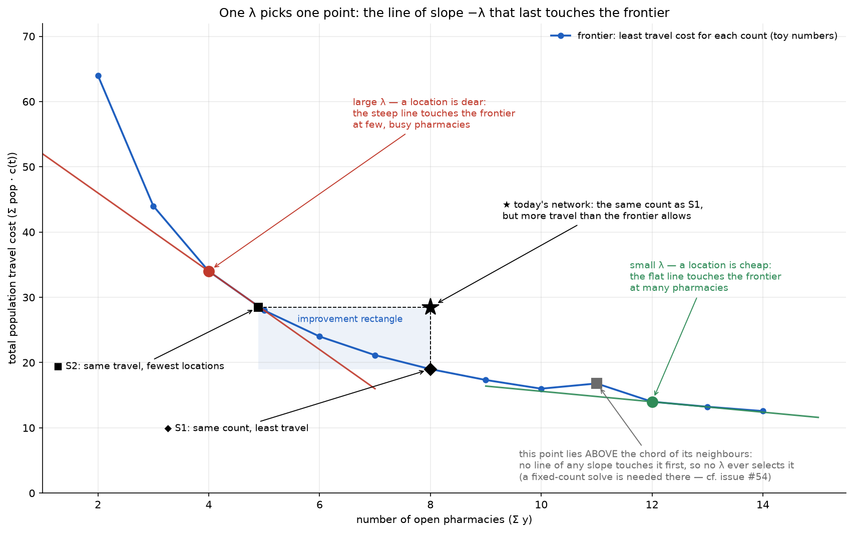
The shaded box is the improvement rectangle (Metrics aggregation and ranking); the price lines are the tangency picture and the grey point a concave dent that no λ can select (issue #54) — both explained on The lambda sweep and the Pareto frontier.
Why count and travel, not λ. λ, the price of one open location (w · €100 000 in the code, the € a placeholder — The lambda sweep and the Pareto frontier), is the knob the sweep turns. Today's count and travel are known, so S1 and S2 mean something whatever a pharmacy really costs; the λ at which the sweep passes each point is reported afterwards as the price that would buy it.
baseline_metrics in lambda_sweep_simplex.jl (around line 167) makes four choices:
-
Nearest by road. Every populated cell goes to the existing pharmacy cell with the smallest travel time in its OD rows; travel cost is
Σ pop · c(t). -
Coverage-consistent pricing. A cell in the candidate-side OD but absent from the existing-side OD can reach no pharmacy today. It is charged BIG — the price the LP pays for leaving a client unserved under soft coverage (Glossary: soft coverage, stranded; The facility location model explained) — times its population, and 120 minutes per resident in time. Before
206923c(6 July 2026) such residents were silently dropped (Denmark ≈ 11 %) and the star sat below the frontier. BIG's value per function (big_cost()= c(120) = 120 for LINEAR, 1.0 for LOGISTIC) and its history from per-area OD maximum to the fixed 120 min (4ec47a9) are on Travel cost functions. -
Cells, not pharmacies.
n_usedcounts the 1 km² pharmacy cells that are the nearest for at least one client; pharmacies sharing a cell count once, a cell nobody is nearest to ("empty"; France has 660 such pharmacies) not at all. Hencefacilities used (cells): 1615 (of 1617)for the Netherlands and its 1 992 pharmacies; S1 targets cells because the candidate side is cells too (Log lines and output files has the units table). -
Raw counts are informational.
RAW_PHARMACY_COUNTS(line 9) holds only"Netherlands" => 1992and adds ann-rawcolumn and a "fewer than raw" line. The NL-only predecessorlambda_sweep.jl(a9ef6cc, 24 May 2026) used 1 992 as the S1 target itself (TARGET_N); the same day (2d1d32b) the target became the cell count and the raw figure stayed as a reference column, "Only NL is known so far". No other country was ever added.
The frontier is a list of solved points, one per grid value of w (1-2-5 per decade: ×2 or ×2.5 per step). Today's count almost never coincides with a solved point, so "the frontier at N" must be constructed, always from a bracket (Glossary): two consecutive solved w values whose counts (S1) or travel (S2) enclose today's value.
Two conventions apply throughout. The count is sum_y (Glossary), the LP's fractional facility count Σ y*; n_open = round(sum_y) is what every rounding must open, so the two differ by under one facility. S1 is bracketed on sum_y because it falls monotonically as λ rises (The lambda sweep and the Pareto frontier), whereas n_open once jumped from 2 296 to 3 894 between w = 0.01 and 0.1 under the old interior-point solver (9ee7ac6, 25 May 2026). The travel is cost_c (Glossary; multi in the deck data), the coverage-honest travel of the multistart rounding, not the LP's lower bound: today's network is a real set of pharmacies and must be compared with another (From LP fractions to real pharmacies).
closest(results, target, key) (driver, around line 504) picks, among all rounded rows (the log's "Combined sweep" table), the one whose sum_y is nearest today's count (S1) or whose cost_c is nearest today's travel (S2); ties go to the lowest w. That row is the printed "scenario summary" and, copied by write_scenario_arrows to the stable S1/S2 folders, the exported location file.
It is coarse: the count moves ~30 % per grid step on average, so the nearest row is typically up to ~15 % off and over 30 % where a ×2.5 step halves the count (SE2 LINEAR −31.6 %, Norway LOGISTIC −27.5 %, SE3 LINEAR +26.4 %). Over 74 sweeps (#52) S1's count was more than 10 % off in 22, median 5.9 %.
A chord (Glossary) is the straight line between two neighbouring solved points; reading the frontier at N means reading that line. The deck tables and chart markers have used chords since cb21c6c (22 July 2026) because a snapped row could sit visibly off the ★ on the chart (SE2 was the example); only interpolation lets a table quote today's exact count. interp in doc/build_deck.mjs (around line 495) takes the pair whose n_open brackets today's count (S1) or whose multi brackets today's travel (S2) and interpolates linearly.
Netherlands, LINEAR, from doc/deck_data.json: 1 615 cells lie between w = 0.2 (1 900 open, 41.59 M) and w = 0.3 (1 334 open, 55.48 M); f = (1 615 − 1 900)/(1 334 − 1 900) = 0.5035, so S1's travel is taken 50.35 % of the way between their travels: 41.59 M + 0.5035 × 13.89 M = 48.59 M person-minutes, −12.1 M (−19.9 %). The λ columns interpolate w on a log scale (the grid is logarithmic, so half-way between grid points means half-way in log w) times €100 000. The λ S1 column brackets on sum_y (1 899.83 → 1 334.42, f = 0.5038) while the Δ column brackets on n_open: λ S1 = 0.2 × 1.5^0.5038 × 100 000 ≈ €24 532, where n_open would give €24 530 — always under one facility apart.
doc/frontier_metrics.py (the rectangle and crossing metrics, Metrics aggregation and ranking) first drops every row that another row beats on both count and travel (rounding noise can produce such rows) and interpolates on the remaining Pareto envelope (Glossary); its λ at the crossing is interpolated linearly in w, unlike every other λ here (reason not recorded). A chord over a convex curve lies slightly above it, so chord S1 savings are mildly under-stated.
Interpolation gives a number, not a network: nobody can map 1 172.5 pharmacies. For the exported files a real solve has to land on the target — bisection (Glossary: solving inside the bracket, repeatedly, keeping the half that still encloses the target).
-
June 2026, S2 only (
b76f643): after the coarse and fine sweeps had finished, bisect the S2 bracket, ≤ 6 solves, 0.5 % early exit — because on the 1-2-5 grid S1 and S2 "collapsed onto the same sweep row" (commit message). -
September 2026, both, inside the loop (
29fcf7f, issue #52):refine_if_closed!(around line 364) runs after every grid point: if the previous and currentsum_yenclose today's count,bisect!runs for S1; if the previous and currentcost_cenclose today's travel, for S2.bisect!(around line 343) solves at the midpoint on a log scale, √(lo·hi), keeps the closest point seen, and stops within tolerance (S1max(1, REFINE_TOL · cells)facilities, S2REFINE_TOL · travel) or afterREFINE_ITERSsolves; eight solves shrink a ×2.5 bracket to ×1.004, a price known to 0.4 %. A scenario within tolerance is pinned (Glossary). Why 0.2 % and 8 rather than June's 0.5 % and 6: not recorded; the one-facility floor is presumably because counts are integers (inference).
Why "the moment the bracket closes" and not after the sweep. HiGHS warm-starts each solve from the basis of the previous one; from a nearby λ that takes seconds, from the half-finished state of a timed-out solve it can take longer than solving from scratch (The lambda sweep and the Pareto frontier). The June bisection ran after the sweep had climbed to w_max, where the last points had timed out, so its first solve timed out too in 14 of 42 LINEAR areas — FRC's LP at w = 0.1 took 75 s as a grid step and hit the 1 h limit when re-solved later (#52): same LP, different starting basis. The same reasoning gives the tail stop (SWEEP_STOP_AFTER_TAIL_FAIL, default 1): the tail (Glossary) — the grid points beyond the S2 bracket, which only extend the frontier for S3 — is cut at the first time-out, because every later point would start from the aborted basis and time out too. The price is a shorter S3 curve for that area.
Refine-only mode. Most areas had a good frontier and only needed S1/S2 re-pinned. SWEEP_STOP_AFTER_REFINE=1 (set by run_resweep_batch.ps1 -RefineOnly) walks the grid from 1e-4, bisects each bracket as it closes and stops — no tail. build_deck_data.py merges its log (logs\refine_<area>_<FUNC>.log) only when it is newer than the sweep log and holds both summaries; a half-finished refine log is ignored and the old snapped rows stay. Since e25416b the walk is LP-only ("light", Glossary) while the previous sum_y is above 1.5 × today's count, skipping 50–100 s of rounding per point against a 7 s LP. A light row has no travel, so an S2 bracket cannot close against it; S2 is then bisected after the walk, from a less favourable basis (inference). Code-level detail: Code walkthrough lambda_sweep_simplex.
Luxembourg LINEAR in #52: refine-only in 35 s; the pinned solve opens 87 cells against today's 86 — inside the one-facility tolerance — where the snapped row had opened 69 (−20 %); S2 within +0.3 % of today's travel.
The instance is the worked example of The lambda sweep and the Pareto frontier: its best networks are all three cells open (2 000 person-minutes), {1, 3} (2 500), {2} alone (5 500) and nothing open (36 000), with break-even prices λ = 500, 3 000 and 30 500. Today's pharmacies are cells {2, 3}: A→2 (20 min), B→2 (10), C→3 (5), so ★ = (2 cells, 100 × 35 = 3 500 person-minutes). The LP is integral at every sweep point below (checked with HiGHS), so each row is one of those four sets.
Sweep on the default grid, columns w · λ · sum_y · travel · n_open · n − cells:
0.001    100   3.0   2000   3   +1
0.002    200   3.0   2000   3   +1
0.005    500   3.0   2000   3   +1   λ = 500 is the 3→2 tie ({1,2,3} and {1,3} both 3 500);
                                     HiGHS, warm-started from 0.002, keeps 3
0.01    1000   2.0   2500   2    0   S1 bracket closes: 3 ≥ 2 ≥ 2, tolerance max(1, 0.002·2) = 1
0.0071   707   2.0   2500   2    0   the one bisection solve, √(0.005·0.01); residual 0: S1 pinned
0.02    2000   2.0   2500   2    0
0.05    5000   1.0   5500   1   −1   S2 bracket closes: 2 500 ≤ 3 500 ≤ 5 500, tolerance 7
All eight S2 midpoints between 0.02 and 0.05 return 2 500 or 5 500 — the frontier jumps at λ = 3 000 — so the log says S2 pinned at w=0.02: cost_c=2500.0 (target 3500.0), 29 % off, and closest exports the same set {1, 3} for S1 and S2: the five-area phenomenon in miniature. On a real area with ~10³ facilities each step moves the count by a few and the bisection converges. A chord (b) would instead report S1 travel 2 500 (−28.6 %) and S2 count 1 + (3 500 − 5 500)/(2 500 − 5 500) = 1.67 — a number, not a network.
In doc/deck_data.json at e25416b the LINEAR scen blocks — where build_deck_data.py stores the snapped summary of (a) — of FRC, FRH, FRJ, FRK and SE2 hold identical S1 and S2 rows. FRK: today 1 685 cells, travel 29.39 M; the grid has w = 0.1 (1 706 open, 24.88 M) and w = 0.2 (1 005, 34.73 M) and nothing between — the June S2 bisection left no row, presumably one of the 14 LINEAR areas whose post-hoc bisection timed out from the far basis (#52; inference, FRK's June log is not in this checkout). closest picks 0.1 on count (21 off versus 680) and on travel (4.5 M short versus 5.3 M over): one row, one file for both. SE2 is worse: with 452 cells between w = 0.2 (637.5 open) and 0.5 (309.25), S1 snaps to 309 locations, 32 % too few, and S2 to the same row.
In-sweep bisection subdivides the bracket until a rounded row lands within 0.2 % of each target. Issue #52's closing comment (commit 216ac77, 12 September — not on GitHub as of 15 September 2026, Branches data and environment) reports the median S1 error down from 5.9 % to 0.13 %, S1 = S2 nowhere, SE2's S1 at 451 of 452. Only country-level Poland LINEAR (3–15 h per solve near S1) keeps its grid point (+1.6 %); its seven NUTS-1 parts are pinned and are what the aggregate uses.
Two limits. Bisection cannot reach a count the integer frontier jumps over: bisect! then returns the closest of its solves and still prints "pinned" — always read the (target …) residual (Denmark LOGISTIC in #52: "pinned" 9.5 % off). And closest ignores which row was pinned — it re-scans all rounded rows, so on a stair-stepped frontier the two exports can still coincide (no reason recorded; closest predates the bisection — inference).
As of September 2026 (e25416b). "→ (c)" means the artefact takes the pinned row once an area has been refined; the deck_data.json in this checkout (last regenerated in de5b178, 3 September) is pre-#52 for every area.
| Artefact | Definition and convention |
|---|---|
| Deck region-slide table (p16–58); p62 and p9 counts | (a) scen row → (c): the snapped row's w, count, fractional y, rounded-vs-LP gap, stranded cells (Deck and charts pipeline) |
| Deck λ tables p60–61 = results page §3 | (b) build_deck.mjs interp; S2 · Δ # is a chord value rounded to whole locations (the CSV keeps 1 172.5 for NL); — = target outside the swept range |
| Deck aggregate table p59 = results page §2 | nearest row of the aggregate curve (aggregate_fd), not interpolated |
| Region-chart markers ◆ ■; λ-axis chart guides (p65–66) | (b) build_charts.py interp_s1_s2 (linear in sum_y / multi); lambda_axis_chart.py crossing
|
doc/frontier_metrics_interp3.csv |
(b) on the Pareto envelope; lambda_cross linear in w
|
S1 / S2 Arrow folders; exported `_<s1 |
s2>_<linear |
| Lambda sweep method §4 | tables (b); "exported files snap … five areas same point" = (a), written before 29fcf7f — history |
| Pharmacy results September 2026 §6 "S1 at 1 334 open (w = 0.300)" | (a); contradicts its own §3, where S1 is at 1 615 by definition |
Never compare a λ-table number with a region-slide table or a location file without checking this matrix: the file holds an integer solve, the table a chord. Netherlands LINEAR in the λ table reads: at today's 1 615 locations, optimal placement saves 12.1 M person-minutes (19.9 %); at today's travel, 443 locations (27.4 %) are surplus; the sweep passes those points at about €24 500 and €34 300 per location.
Native units first, € second. The tables lead with Δ person-minutes (or Δ logistic cost plus mean minutes) and Δ locations, with λ afterwards in grey — a REGIO-review outcome (doc/deck_changes_from_review.md §1 and §5, comments by Ana Moreno Monroy, Martijn Brons and Bernhard Nöbauer; b3c634b, 4 September 2026; Decision log): the frontier answers "by how much" without λ, and changing the €100 000 placeholder moves only the € labels.
export_s1s2_locations.jl reads NewPharmacies\<area>\lambda_sweep\<FUNC>\<S1|S2>\assignment.arrow (id, open), keeps open == 1, joins the ids to that area's own <area>_j.arrow for x, y, and writes <area>_<s1|s2>_<linear|logistic>_open.arrow (EPSG:3035, one row per open location). Windows ignores case in file names but Linux does not, so the exporter writes the lower-case names that services_allocated expects (#45).
GeoDMS reads the stable S1/S2 folders back through ReadSweepResults_T for map views (lin_S1, lin_S2, log_S1, log_S2; per-client minutes saved as dT_*); the names are stable because each area's S1/S2 sit at a different w, so a hard-coded w in the .dms fitted one area only (df4febf, 3 June 2026). Separately, Chris's services_allocated reads the exported *_open.arrow files for his own reporting (LOGISTIC only, 21 areas). Item by item: GeoDMS OD matrix and choice set.
| What | Where (e25416b) |
|---|---|
| Baseline ★ |
lambda_sweep_simplex.jl → baseline_metrics, write_baseline_arrows (L58), RAW_PHARMACY_COUNTS (L9); settings.jl → big_cost (L97) |
| Bracket tests |
crosses (L341), find_bracket
|
| Bisection and the light walk |
bisect!, refine_if_closed! (L364), grid loop (L385–415), fallback bisection (L474–490); design note in the comment block L316–334 |
| Basis restore, LP-only solve |
lp_run.jl → resolve_for_basis!, solve_at_w!(…; rounding=false) (L460) |
| Snapped selection, stable folders |
closest, write_scenario_arrows (L47), summary block (L514–548) |
| Chord interpolation |
doc/build_deck.mjs → interp; doc/build_charts.py → interp_s1_s2 (L38); doc/lambda_axis_chart.py → crossing (L59); doc/frontier_metrics.py → interp_y_at_x, interp_x_at_y, interp_w_at_x (L49–87) |
| Refine-log merge |
doc/build_deck_data.py (L169–183) |
| Export and read-back |
export_s1s2_locations.jl; cfg/main/Analyses.dms → ReadSweepResults_T (L219), SweepResults (L377); cfg/main/SourceData/Locations.dms → services_allocated (L500) |
The function-by-function walk is Code walkthrough lambda_sweep_simplex; running a refine-only pass is in Running a sweep end to end.
| Name | Default | What it changes | Why you would change it | Interactions |
|---|---|---|---|---|
REFINE_TOL |
0.002 |
bisection tolerance: S1 max(1, tol · cells) facilities, S2 tol · travel
|
tighter pins cost solves; looser on an area whose solves take hours (why 0.2 % replaced June's 0.5 %: not recorded) | capped by REFINE_ITERS
|
REFINE_ITERS |
8 |
max solves per bisection | rarely; 8 halvings reach ≈ ×1.004 in w (why 8 replaced June's 6: not recorded) | a jump in the integer frontier uses all 8 |
SWEEP_STOP_AFTER_REFINE |
0 |
1 = refine-only: light walk, stop once both pinned |
re-pin S1/S2 without re-sweeping the tail | set by -RefineOnly; log must be refine_… for build_deck_data.py
|
SWEEP_STOP_AFTER_TAIL_FAIL |
1 |
end the sweep at the first failure after both are pinned |
0 to keep trying the tail (each try may burn LP_TIME_LIMIT) |
full sweeps only |
-
"Pinned" is not "exact". Read the
(target …)residual. The acceptance checkdoc/check_s1s2.pynamed in #52 is not in this checkout. -
mean_tis not coverage-consistent. The baseline charges stranded residents 120 min, a sweep row'smean_tcounts them at 0 min;cost_cis consistent — the units table on Log lines and output files. -
S1/S2folders are overwritten by every run, refine-only or partial;w=<float>folders accumulate and nothing cleans them. -
Stale wiki sentences. Lambda sweep method §4 (snap, five areas) and Pharmacy results September 2026 §6 (the 1 334 row) were true when written at midday on 10 September (12:46, 13:55) and superseded by
29fcf7fande25416bthat evening (18:09, 20:06). - Where the choice-set radius binds (SE2, ITF), S2 under-counts the surplus — Scope rules and data gaps. An exact fixed-count MIP (Glossary: the integer programme, not its relaxation) is the roadmap's answer to both the chord bias and the integrality gap.
-
The post-
e25416brefinements (6aaab27,92ab4e4,82d84b4,86e242e) are unpushed — see Branches data and environment; this page documentse25416b.
- Lambda sweep method · Pharmacy results September 2026 · The lambda sweep and the Pareto frontier · From LP fractions to real pharmacies · Metrics aggregation and ranking · Code walkthrough lambda_sweep_simplex · Log lines and output files · Deck and charts pipeline · GeoDMS OD matrix and choice set · Running a sweep end to end · Decision log · Scope rules and data gaps · Branches data and environment · Background theory · Glossary