Repository navigation
Pharmacy results September 2026
Headline results from the deck
doc/lambda_sweep5.pptx
(Dekhuijzen & Hilferink, draft for discussion, September 2026). Method on Lambda sweep method.
Every figure below has a LOGISTIC twin in the deck; unless stated, numbers are LINEAR.
Not comparable with earlier decks. Two method changes — landbody-complete networks and NUTS region exclusion — change which residents are counted, so baselines, frontiers and the ranked lists all shifted (deck p8, p63).
Catchment = residents whose nearest pharmacy by road travel time is this one (a cell's catchment
split evenly among the pharmacies in it). Per country (deck p3, doc/pharmacy_descriptives.csv):
| country | pharmacies | residents | resid./pharm. | #empty | p10 | p50 | p90 | max |
|---|---|---|---|---|---|---|---|---|
| Austria | 1 467 | 8.9 M | 6 088 | 3 | 2 422 | 5 666 | 10 203 | 25 354 |
| Belgium | 4 860 | 11.5 M | 2 373 | 11 | 961 | 2 137 | 4 053 | 10 019 |
| Denmark | 536 | 5.8 M | 10 736 | 0 | 4 892 | 10 014 | 17 801 | 35 188 |
| France | 20 698 | 65.3 M | 3 155 | 660 | 1 182 | 2 869 | 5 495 | 17 502 |
| Italy | 12 991 | 58.7 M | 4 520 | 56 | 1 040 | 3 160 | 9 107 | 85 669 |
| Lithuania | 1 253 | 2.8 M | 2 240 | 0 | 671 | 1 782 | 4 507 | 13 754 |
| Netherlands | 1 992 | 17.5 M | 8 765 | 4 | 2 661 | 7 952 | 15 567 | 33 497 |
| Norway | 1 057 | 5.1 M | 4 835 | 5 | 1 661 | 4 300 | 8 548 | 23 011 |
| Poland | 13 791 | 37.1 M | 2 688 | 3 | 878 | 2 280 | 5 017 | 19 078 |
| Portugal | 2 801 | 10.3 M | 3 680 | 16 | 1 262 | 2 941 | 6 497 | 19 709 |
| Sweden | 1 448 | 10.2 M | 7 078 | 5 | 2 098 | 6 208 | 12 659 | 37 107 |
#empty = pharmacies that are never the road-nearest for any populated cell. The same table per
1 km² location (cells with ≥ 1 pharmacy) and for the FR/IT/SE NUTS-1 regions: deck p4–6.
The within-country spread is wide everywhere — the Netherlands alone runs from 4 394 (p10) to
34 905 (max) residents per location — which is why fixed min/max catchment caps were dropped.
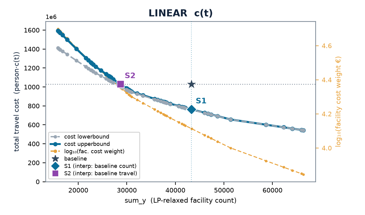
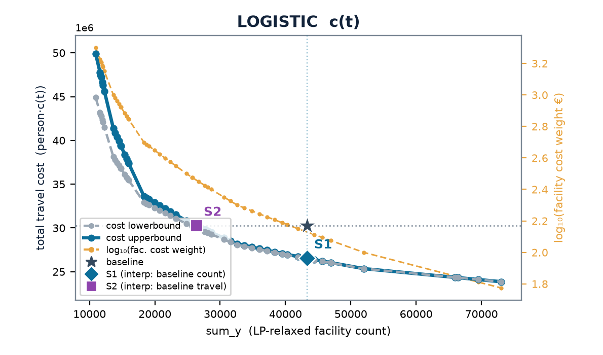
Facilities and travel cost summed per λ over the 41 disjoint areas (exact by separability). Aggregate baseline travel: LIN 1 030 M person-minutes, LOG 30.3 M.
| point | w | locations | Δ locations | multi vs relax | Δ travel | |
|---|---|---|---|---|---|---|
| LINEAR | S1 same count | 0.130 | 43 357 | +0 % | +0 % | −26 % |
| S2 same travel | 0.227 | 28 609 | −34 % | +3 % | +0 % | |
| fewest facilities swept | 0.500 | 15 808 | −64 % | +13 % | +55 % | |
| most facilities swept | 0.0001 | 433 828 | +901 % | +0 % | −93 % | |
| LOGISTIC | S1 same count | 0.00130 | 44 416 | +3 % | +0 % | −13 % |
| S2 same travel | 0.00282 | 26 673 | −38 % | +1 % | −0 % | |
| fewest facilities swept | 0.0200 | 10 933 | −75 % | +11 % | +65 % |
Read: relocating today's pharmacies without adding any would cut population travel by about a quarter (linear); holding travel where it is, about a third of the locations are surplus. The Δ columns are native units and need no λ; λ only prices them (placeholder €100 000 per location).
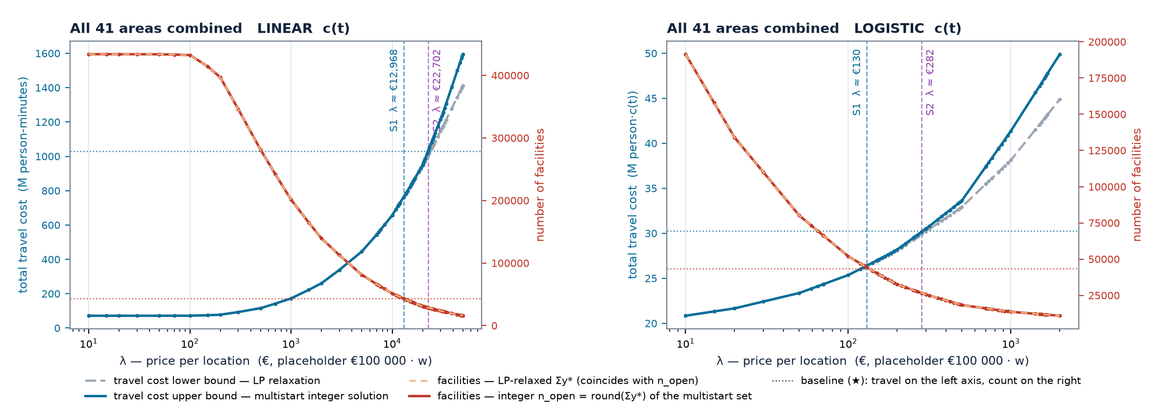
The frontier hides λ. Read along it instead — λ on a log axis, the two travel-cost bounds on the left
(LP relaxation below, multistart integer solution above), the facility count on the right — and the
sweep's dynamics show: the count collapses over two decades of λ (LINEAR: from ~433 000 below €100
per location to ~43 000 at S1) while the travel bounds stay on top of each other, and they separate
only near S2. The dotted lines are the baseline, so S2 is where travel crosses its baseline and S1
where the count crosses its. The two count curves coincide by construction (n_open = round(Σy*)):
the certified bound is on total cost, not on the count, so the informative gap is the one on the
left axis. Under LOGISTIC the whole picture is compressed into λ ∈ [€10, €2 000] — the degeneracy of
deck p64. Deck p65; the Netherlands version is p66:
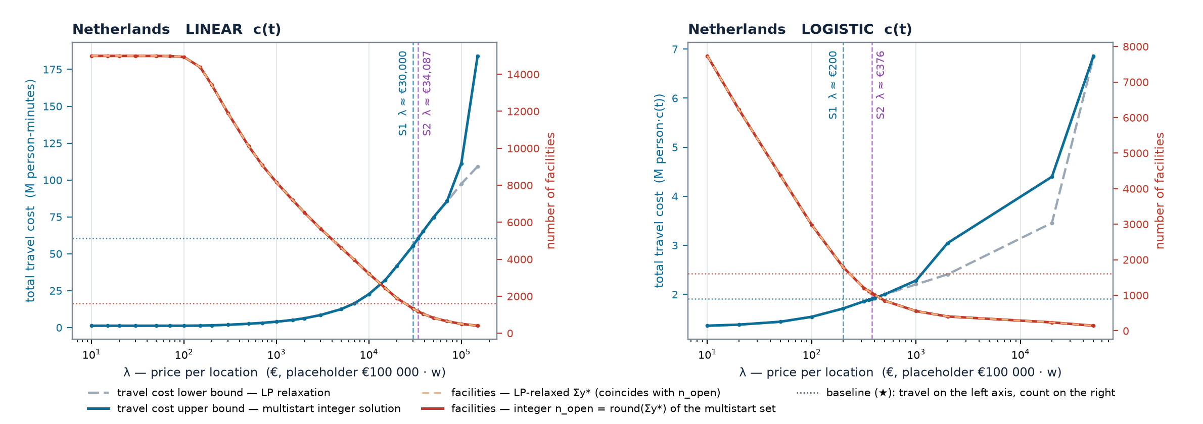
Under LINEAR the Netherlands bounds open only above ~€50 000 per location, beyond S2, so its S1/S2
figures sit where lower and upper bound agree. Any area: python doc/lambda_axis_chart.py <REGION>.
Gains read off the multistart frontier by interpolation between adjacent sweep points; λ is the
price per location at which the sweep reaches that point (deck p60–61,
doc/frontier_metrics_interp3.csv).
| country | today # | S1 · Δ travel (lin) | S2 · Δ # (lin) | S1 · Δ cost · Δ mean t (log) | S2 · Δ # (log) | λ S1 lin | λ S2 lin |
|---|---|---|---|---|---|---|---|
| Netherlands | 1 615 | −12.1 M min · −19.9 % | −443 · −27.4 % | −8.0 % · −0.7 min | −551 · −34.1 % | 24 532 | 34 329 |
| Luxembourg | 86 | −427 k min · −17.8 % | −26 · −29.9 % | −7.6 % · −0.7 min | −30 · −35.1 % | 15 945 | 25 641 |
| Estonia | 292 | −1.3 M min · −22.6 % | −94 · −32.3 % | −13.4 % · −0.9 min | −121 · −41.4 % | 11 388 | 19 421 |
| Latvia | 496 | −1.5 M min · −19.9 % | −144 · −29.1 % | −11.3 % · −0.8 min | −183 · −36.8 % | 8 822 | 14 262 |
| Slovenia | 306 | −1.5 M min · −13.1 % | −82 · −26.7 % | −9.0 % · −0.8 min | −99 · −32.4 % | 17 680 | 25 450 |
| Lithuania | 582 | −2.9 M min · −23.5 % | −204 · −35.1 % | −14.4 % · −1.0 min | −268 · −46.0 % | 10 987 | 19 834 |
| Ireland | 862 | −4.0 M min · −16.9 % | −235 · −27.2 % | −8.8 % · −0.7 min | −297 · −34.5 % | 14 269 | 21 020 |
| Norway | 755 | −10.3 M min · −25.3 % | −326 · −43.2 % | −18.0 % · −1.8 min | −359 · −47.6 % | 23 174 | 49 999 |
| Denmark | 466 | −5.5 M min · −14.8 % | −133 · −28.6 % | −11.0 % · −0.9 min | −166 · −35.6 % | 37 082 | 55 960 |
| Austria | 1 129 | −8.8 M min · −20.4 % | −373 · −33.0 % | −13.3 % · −1.0 min | −497 · −44.0 % | 18 361 | 31 027 |
| Portugal | 1 882 | −7.4 M min · −21.6 % | −527 · −28.0 % | −8.3 % · −0.7 min | −623 · −33.1 % | 10 473 | 17 033 |
| Czechia | 1 624 | −8.8 M min · −19.8 % | −487 · −30.0 % | −8.9 % · −0.7 min | −587 · −36.1 % | 14 550 | 22 885 |
| Belgium | 2 958 | −3.2 M min · −14.9 % | −520 · −17.6 % | −3.0 % · −0.3 min | −552 · −18.7 % | 5 666 | 7 340 |
| Poland | 7 027 | −23.7 M min · −17.8 % | −1 883 · −26.8 % | −7.5 % · −0.6 min | −2 207 · −31.4 % | 10 254 | 15 809 |
Selected NUTS-1 regions (all 28 in the deck):
| region | today # | S1 · Δ travel (lin) | S2 · Δ # (lin) | λ S1 lin | λ S2 lin |
|---|---|---|---|---|---|
| FR1 · Île-de-France | 1 449 | −2.9 M min · −23.0 % | −218 · −15.1 % | 11 918 | 16 444 |
| FRI · Nouvelle-Aquitaine | 1 584 | −2.4 M min · −8.7 % | −296 · −18.7 % | 8 368 | 10 901 |
| ITC · Nord-Ovest | 2 890 | −15.6 M min · −33.7 % | −1 101 · −38.1 % | 10 511 | 20 047 |
| ITF · Sud | 1 253 | −40.7 M min · −45.8 % | −732 · −58.5 % | 30 189 | 101 789 |
| ITG · Isole | 891 | −15.0 M min · −49.1 % | −474 · −53.2 % | 18 626 | 56 207 |
| SE1 · Östra Sverige | 388 | −4.8 M min · −21.9 % | −143 · −36.9 % | 27 492 | 44 267 |
| SE2 · Södra Sverige | 452 | −6.0 M min · −18.5 % | −167 · −36.9 % | 33 567 | 57 265 |
| PL8 · Wschodni | 1 065 | −4.0 M min · −17.3 % | −282 · −26.5 % | 10 273 | 16 347 |
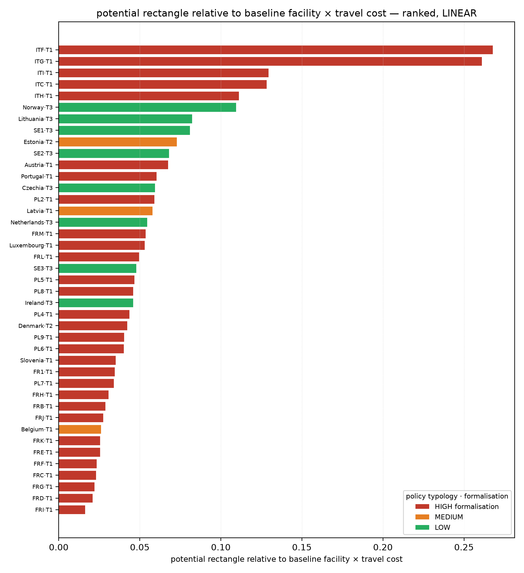
The improvement rectangle (baseline ↔ S1 ↔ S2) relative to baseline count × travel. Southern
Italy stands far above the field — ITF 0.268, ITG 0.261 — followed by the other Italian regions
(ITI 0.129, ITC 0.128, ITH 0.111), Norway (0.109), Lithuania, SE1 and Estonia; the French regions
and Belgium close the list (FRI 0.016). Under LOGISTIC the top is the same (ITF 0.177, ITG 0.160,
Norway 0.086, SE1 0.071).
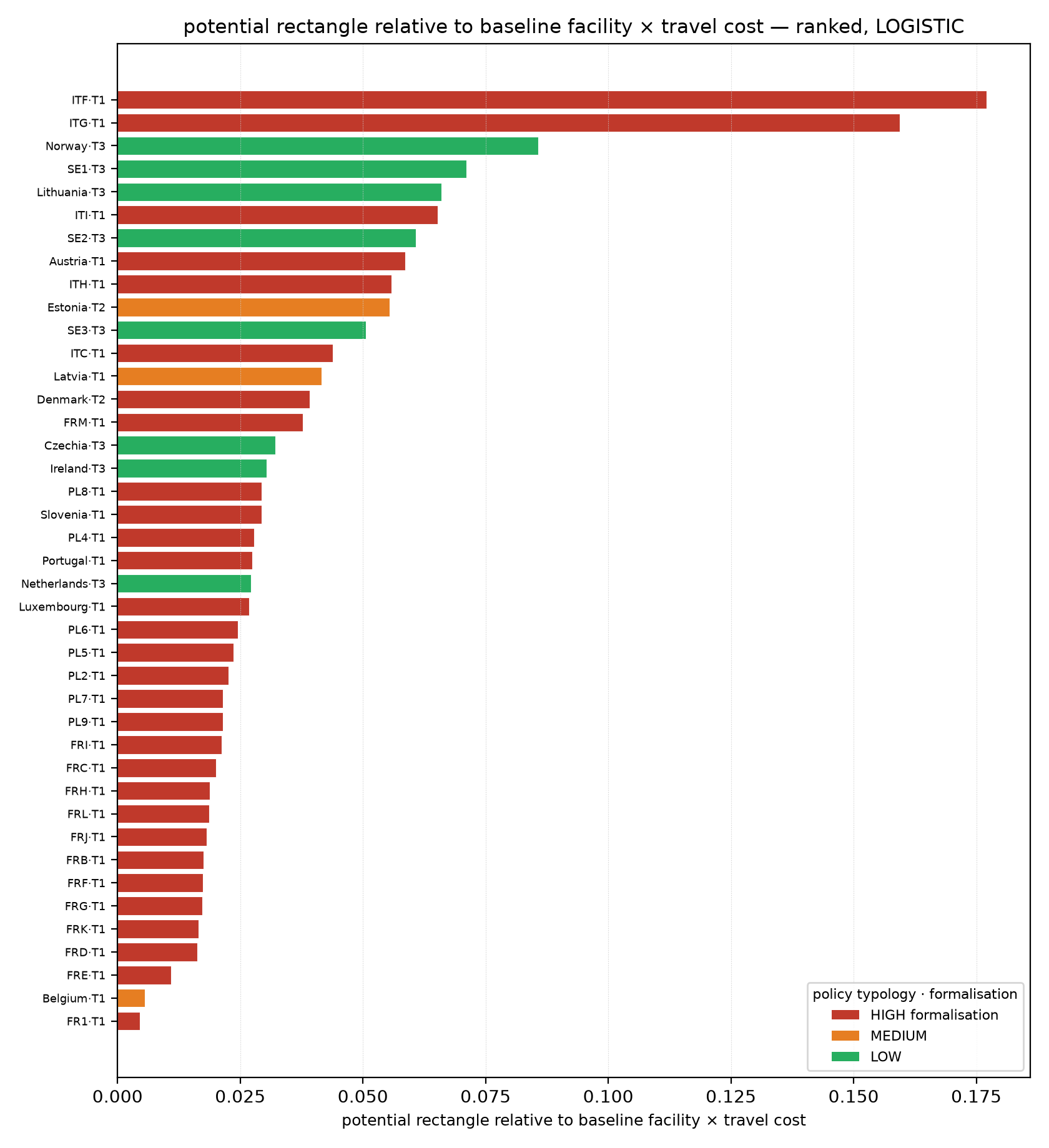
Bars are coloured by the pharmacy-regulation typology (formalisation level; T1 rule-of-law-
anchored, T2 consensual-pluralist, T3 public-interest majoritarian). The gaps do not follow
regulatory regime: the largest span both high-formalisation systems (Italy, Portugal, PL8) and
low-formalisation ones (Sweden, Norway, the Netherlands) — geography dominates regime. The ranking
is free of coverage artefacts: ITF ranks first on an unchanged value after the two scope rules.
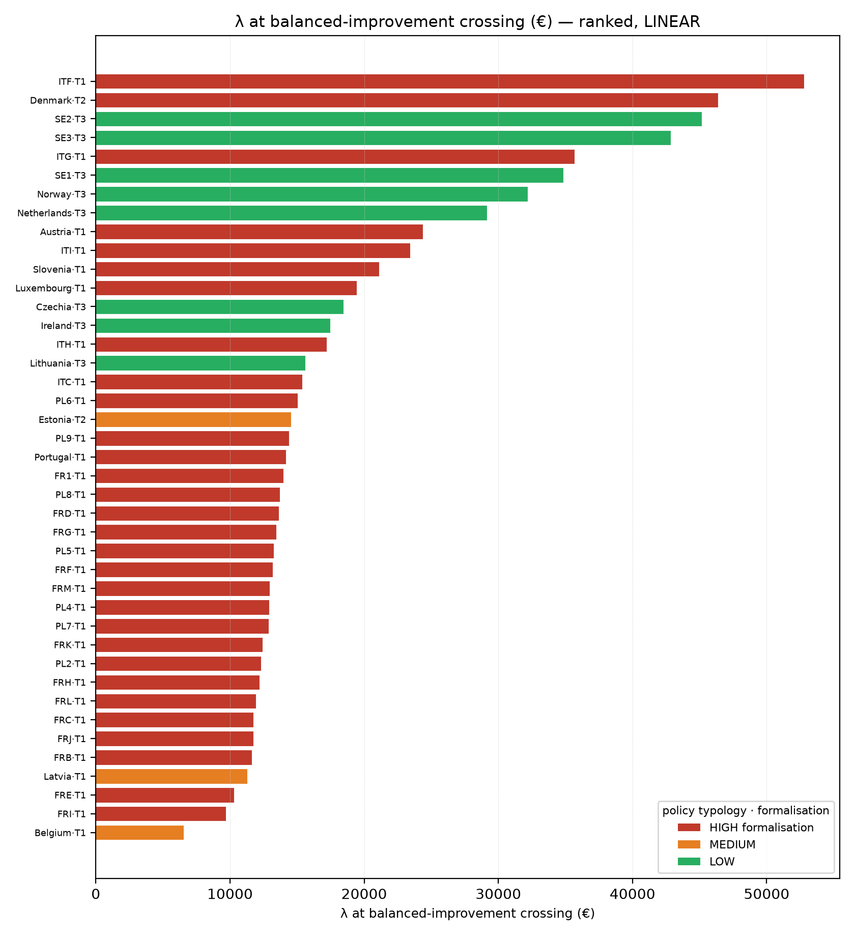
λ at the diagonal crossing — the price per location at which the balanced improvement is the optimum — ranks ITF (52 807), SE2 (45 168), ITG (35 671), SE1 (34 859) and Norway (32 176) highest, Belgium and FRI lowest. In € only through the placeholder; the crossing and the order do not depend on it.
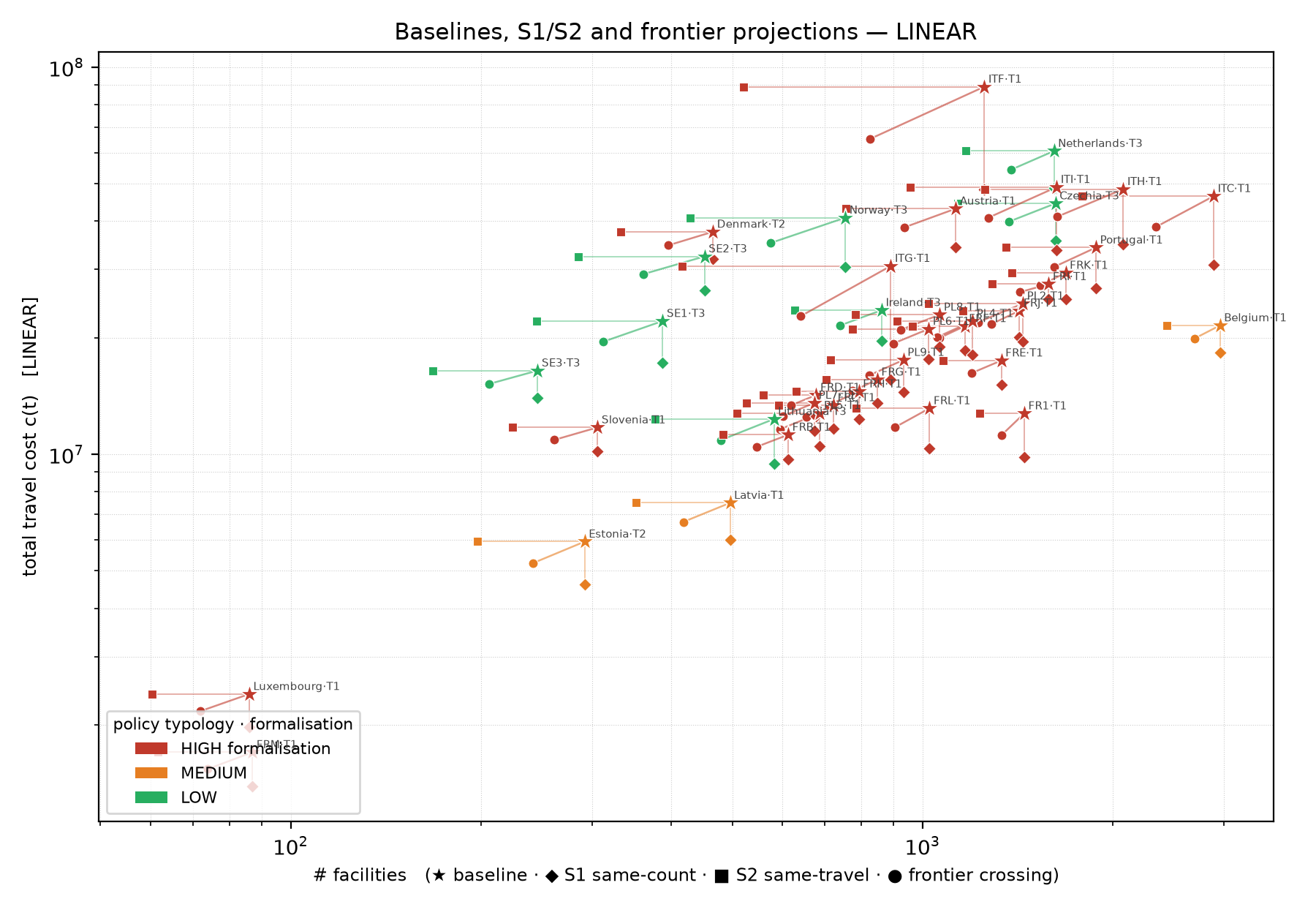
The multistart upper bound sits +0–18 % above the LP lower bound under LINEAR and +0–4.7 % under LOGISTIC (deck p62). For most areas the two are now nearly a line; rounding costs most where stranding is dear, and the sparse Swedish regions keep the largest gaps (SE2: 56 clients stranded by rounding at S1 under LINEAR; SE3: 130 under LOGISTIC). ITF S2 is the one area with a +3 % gap.
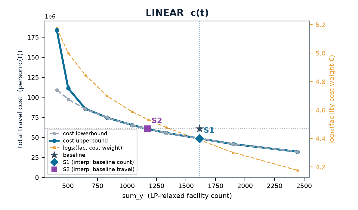
Grey dashed = LP lower bound, blue = multistart upper bound, amber = log₁₀ λ (right axis); ★ today, ◆ S1, ■ S2. Netherlands LINEAR: 1 615 cells today, 3.48 min mean travel; S1 at 1 334 open (w = 0.300), S2 at 1 180 open (w = 0.341), both at +0 % over the bound.
Editor's note (15 Sep 2026). "S1 at 1 334 open" is the snapped sweep row nearest today's count (
doc/deck_data.json,scen.S1, w = 0.3), the row the exported files and chart markers use — not the S1 of the table in §3, which is chord-interpolated at today's 1 615 cells (S1 bracket: w = 0.2 with 1 900 cells … w = 0.3 with 1 334). S2 at w = 0.34087 is a bisection point. Which artefact uses which definition: Scenarios S1 S2 S3.
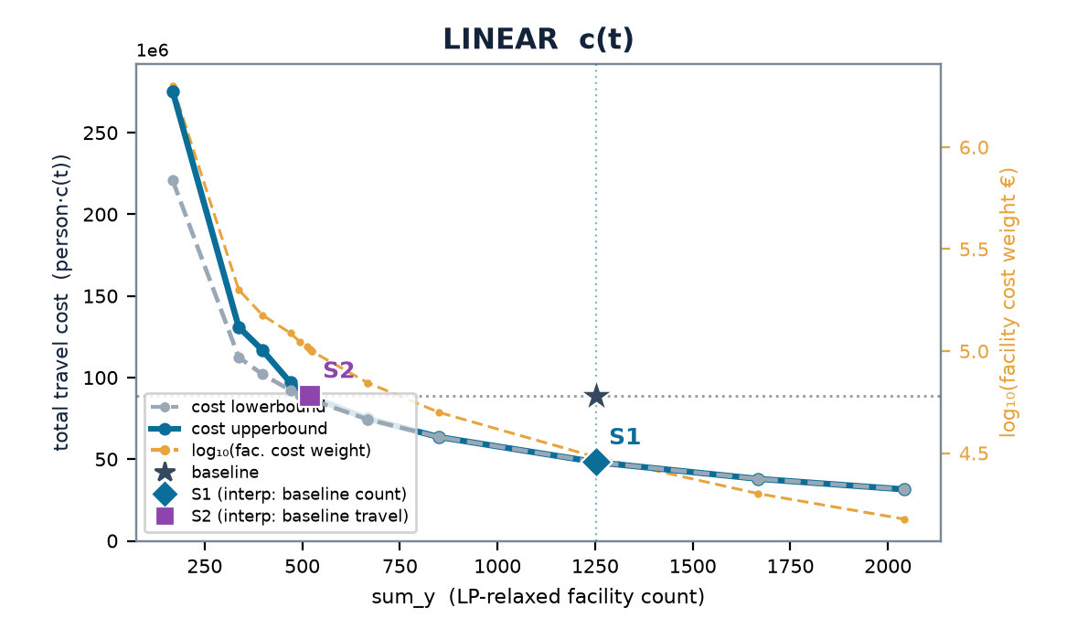
ITF, the area with the most to gain: the frontier lies far below the baseline star.
Decisions sought from the group: the travel-cost shape (linear vs logistic, and whether to rescale the logistic to match the linear at 0 and 60 min); widening the candidate radius before RSSV; territorial coverage constraints for equity, or keeping soft coverage.
Remaining, in priority order: communicate λ intuitively (person-minutes per location); widen the candidate radius per client (5 → 10 nearest existing), one area first; RSSV spatial-voting candidate reduction; an exact soft-coverage p-median MIP to pin S1/S2 at the baseline count; territorial coverage constraints; the logistic rescaling decision; calibrate the real fixed cost; capacity caps; counterfactuals.
Not pursued (decided 4 September 2026): the catchment-cap / min-threshold ladder; age-weighted demand; candidate cells plus their neighbours; urban/non-urban split and a settlement candidate set; flat-then-linear cost and logit-parameter sensitivity; pharmacist-based and pooled caps.