Rendering
Everything drawn for this panel is a 640×48 SkiaSharp surface, copied to the device as BGRA with an ordered dither applied on the way out.
SKCanvas → SKBitmap (Bgra8888) → dither → 121 HID writes
There is no channel swap. SkiaSharp's Bgra8888 layout on a little-endian
machine is byte-for-byte the panel's wire order, so the surface's pixel span is
the upload buffer.
At 24 fps the budget is 41.7 ms; at 30 fps it is 33.3 ms. Measured per-frame cost on real hardware is 15.1–18.4 ms, essentially all of it the 121 HID writes. That leaves roughly half the budget for drawing, which is a lot — all 32 visualizer modes hold 30 fps exactly, including the ones that touch every pixel every frame.
Two rules keep it that way.
SkiaSharp objects wrap native memory the GC cannot see, so an undisposed one
leaks with zero GC pressure — no memory warning, no collection, nothing to
suggest a problem until the process is killed. An SKPathBuilder created per
frame in one chart routine leaked about 192 objects a second and eventually got
the editor OOM-killed.
Paints, shaders, bitmaps and point arrays are all allocated once and reused. Note
that Detach() does not dispose the builder.
SKBitmap.SetPixel is a managed→native call per pixel. At 640×48 that is 30720
of them per frame, and it measurably missed the frame target — 27.7 fps against
30 while every other mode made 30.0 exactly.
Full-pixel effects compose into a byte[] and push it with a single
Marshal.Copy. Same output, back to 30.0 fps.
The whole display is 48 px tall. For a meter with a 60 dB range that is 1.25 dB per pixel, which changes what is worth drawing:
- Peak caps carry more information than bar height does. A transient that moves a bar by two pixels moves a cap to a position that stays put and can be read.
- Auto-ranging beats fixed scale, which reverses the obvious choice. A fixed 20–95 °C scale renders a drive moving 36.8→37.1 °C as one fifth of a pixel, so every chart is a flat line. Auto-ranged, the same four degrees travel thirteen pixels. Magnitude is not lost, because the reading and its min/max are printed next to the chart.
- A floor on the auto-ranged span is required, or a perfectly still sensor has its last digit of noise stretched to full height and looks like a seismograph.
- Effects ported from full-screen visualizers carry constants tuned for hundreds of rows. The classic fire routine subtracts 1–2 per row, which is right over 300 rows and leaves a 255 seed still at ~192 after 48 — every pixel lit, no flame tip, a formless wash. Derive falloff from the height.
Two constraints stack: the panel is 18-bit, and its green primary is yellow-shifted (see The Panel).
- Gradients are dithered with an 8×8 ordered Bayer matrix, scaled to exactly the two bits the panel discards. Ordered, not error-diffused, so a static display does not shimmer.
- Segmented and near-binary designs avoid the quantisation entirely, which is a real reason to offer them rather than a nostalgic one.
- Every palette is provisional until it has been seen on the glass.
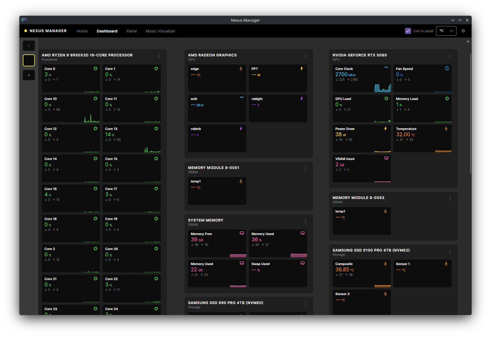
Every sensor the machine reports, discovered rather than listed. 78 across seven devices on this desktop.
The strip is divided among cells — sensor readouts, touch buttons and visualizers — which all share one weight budget. A screen with four readouts and one button gives the button a fifth of the strip, not half.
Lead and trail weights are part of the same budget, so a screen using fewer cells leaves the remainder as background rather than stretching one cell edge to edge. A single cell has no neighbour to drag against, which is the practical reason the gaps exist at all.
One inherited wart, documented because it is visible: cells are laid out grouped by type, so a readout cannot sit between two buttons. Ordering is fixed by type rather than by the configuration.