Example

Example

A small simulated dataset, bundled with BACoN, to check an installation and to see every output in a few seconds. example/make_example.py generates it (standard library only; the same files every time):

• an annotated 30 kb circular reference ("organelle"), as fasta and as GenBank;
• four samples of about 50x of simulated Nanopore reads (1–20 kb, 1.5% errors), each mixed with 20% of reads from an unrelated sequence that baiting must remove;
• known SNPs, in chosen genes and contexts: alpha is identical to the reference, beta has 6 SNPs, gamma has beta's 6 and 4 more, delta has 10 of its own;
• a sample metadata file with simulated values.

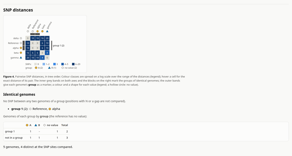
	Reference	alpha	beta	gamma	delta
Reference	0	0	6	10	10
alpha	0	0	6	10	10
beta	6	6	0	4	16
gamma	10	10	4	0	20
delta	10	10	16	20	0

The reference

The reference is laid out like a plastome, with a real inverted repeat (IRa is the reverse complement of IRb):

Region	Coordinates	Length
LSC (large single copy)	1–16,000	16,000 bp
IRb (inverted repeat)	16,001–19,000	3,000 bp
SSC (small single copy)	19,001–27,000	8,000 bp
IRa (inverted repeat)	27,001–30,000	3,000 bp

It carries 23 synthetic genes. Every name is made up (nothing comes from a real organism): 15 protein-coding genes orf01–orf15, open reading frames of random sense codons (ATG, no internal stop, a stop codon) of 300 to 1,500 bp on both strands, orf04 being split by a 500 bp intron (join(4201..4600,5101..5699)); four tRNA genes trnA-sim–trnD-sim and an rRNA gene rrn16-sim (1,500 bp); the rRNA gene and trnD-sim lie in the inverted repeat, so each appears twice, on opposite strands; and a pseudogene orf03-ps, a truncated, diverged copy of the start of orf03. The rest is random sequence (37% GC).

data/reference.gb is the GenBank record: LOCUS (circular), VERSION organelle, DEFINITION simulated circular reference, a source, two repeat_region features (/rpt_type=inverted, /standard_name="IRb" and "IRa"), and for each gene a gene feature with its CDS (/codon_start=1, /transl_table=11, /translation), tRNA or rRNA, or /pseudo. data/reference.fasta is the same sequence as fasta, with the header organelle simulated circular reference: byte for byte what BACoN writes to reference.fasta from the GenBank file, so the GenBank file could be given as -r instead of the fasta and --annotation.

The 20 SNPs are planted outside the inverted repeats (both copies stay identical in every genome), at least 40 bp apart, in chosen contexts: 12 in coding sequences (5 synonymous, 6 missense, 1 nonsense; on both strands, one in the second exon of orf04), 1 in the intron of orf04, 2 in tRNA genes, 1 in the pseudogene and 4 in intergenic spacers. data/planted_snps.tsv lists the positions of each sample and data/planted_effects.tsv the expected region, gene, context, codon change and effect of each SNP, computed by the generator without BACoN:

position  ref  alt  samples     region  gene      context    codon    amino_acid  effect
573       T    C    beta,gamma  LSC     orf01     CDS        AAT>AAC  N91N        synonymous
931       A    C    delta       LSC     orf01     CDS        AAC>CAC  N211H       missense
2440      G    T    beta,gamma  LSC     orf02     CDS        CGC>AGC  R121S       missense
3457      C    T    delta       LSC     orf03     CDS        CGA>TGA  R153*       nonsense
4851      C    A    beta,gamma  LSC     orf04     intron
5400      A    C    beta,gamma  LSC     orf04     CDS        AAA>CAA  K234Q       missense
...

data/metadata.tsv is a sample metadata file (Usage) with the columns group (A, B, and no value for delta), year, origin and a free-text note; its first lines, starting with # before the header, are comments saying that the values are simulated.

Running it

conda activate BACoN
bash example/run_example.sh example_output      # optional: number of threads as a second argument

The script generates the data in example_output/data/, runs BACoN with the default settings, the annotation and the metadata into example_output/bacon/:

bacon -r example_output/data/reference.fasta -i example_output/data/reads -o example_output/bacon \
    --annotation example_output/data/reference.gb --metadata example_output/data/metadata.tsv

and checks the results against the truth: the SNP distances (table above), the region, gene, context and effect of every SNP of the VCF (planted_effects.tsv), and that the report shows the annotation and the metadata. It exits with an error if anything differs:

OK: all 6 pairwise SNP distances match the truth (example_output/bacon/4_compared/ska/snp_distances.tsv)
OK: the 20 SNPs are annotated as planted (12 coding changes: 5 synonymous, 6 missense, 1 nonsense)
OK: report.html has the annotation and the metadata (example_output/bacon/report.html)

The whole script takes about 7 seconds with 8 threads (5 of them to simulate the reads).

The report

Open example_output/bacon/report.html in a browser. The report of this example is also online: view it or download it. (Local paths were removed from it before publication: the program paths start with $CONDA_PREFIX.)

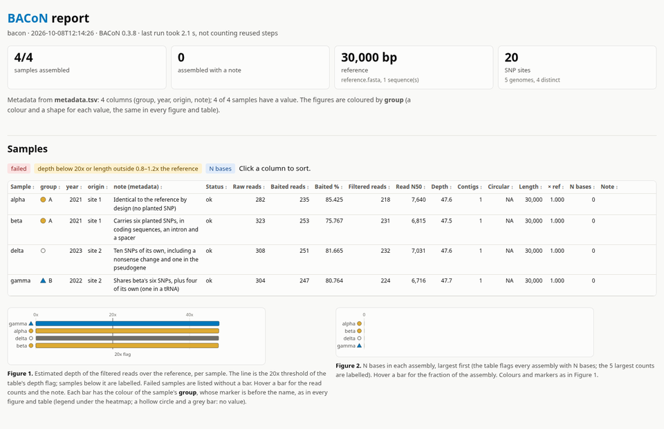
Overview and samples. All four samples assembled: 235 to 253 of the 282 to 323 reads of each sample matched the reference (the others are the off-target reads), and after filtering the depth is 47.5–47.7x (Figure 1). The templated assembly is 30,000 bp for each sample, as long as the reference, with no N base (Figure 2): the reads span the 3 kb inverted repeat, so the consensus is called in both copies. The samples table has the metadata columns after the sample name; group colours the figures, so its values carry their marker.

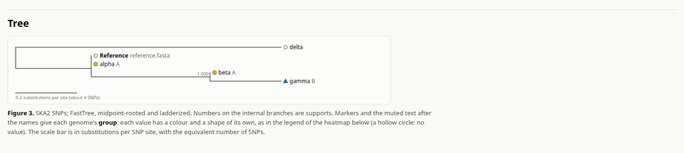
Tree. alpha sits with the reference; beta and gamma form a clade (their 6 shared SNPs); delta is on its own branch. Each leaf gets the marker of its group, a colour and a shape (A a circle, B a triangle), and the group after its name; delta, without a value, gets a hollow circle.

SNP distances. The heatmap, in tree order, shows the pairwise distances; the reference and alpha form a group of identical genomes (the inner grey band and the block on the right), and the outer band gives the group of each genome. Under the list of identical genomes, a table counts, for each group of identical genomes, the genomes of each value of group.

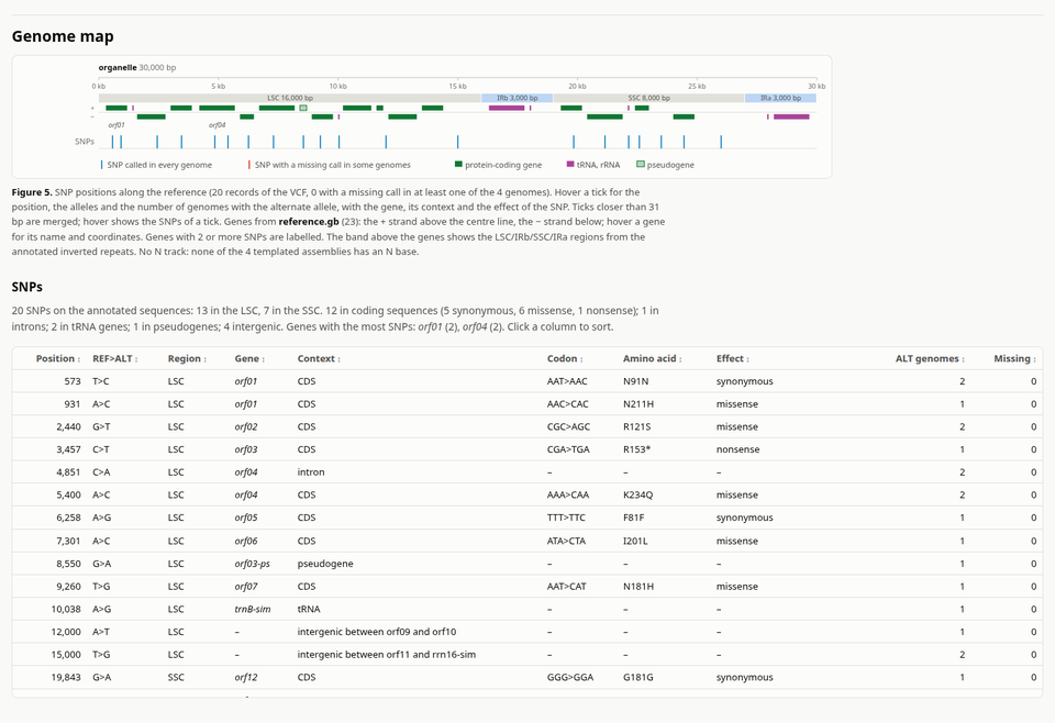
Genome map and SNPs. example_output/bacon/4_compared/ska/snps.vcf lists the 20 planted SNPs at their positions in the reference, with the genotype of each sample. The genome map shows them over the 23 genes of reference.gb (the + strand above the centre line, the − strand below; orf01 and orf04, with 2 SNPs each, are labelled) and the LSC/IRb/SSC/IRa band derived from the annotated inverted repeats (the example's 3 kb repeat is below the 5 kb minimum of the detection in the sequence, so the band needs the annotation); hovering a tick gives the alleles, the gene, the context and the effect. Every genome has a call at each SNP, and no assembly has an N base, so there is no N track. The paragraph under the map sums it up:

20 SNPs on the annotated sequences: 13 in the LSC, 7 in the SSC. 12 in coding sequences (5 synonymous, 6 missense, 1 nonsense); 1 in introns; 2 in tRNA genes; 1 in pseudogenes; 4 intergenic. Genes with the most SNPs: orf01 (2), orf04 (2).

and the SNP table lists each SNP with its region, gene, context, codon and amino-acid change and effect: for example position 3,457 C>T in orf03, CGA>TGA, R153*, nonsense (delta only), or position 5,400 A>C in the second exon of orf04, AAA>CAA, K234Q, missense (beta and gamma). Every row agrees with planted_effects.tsv; the script checks it.

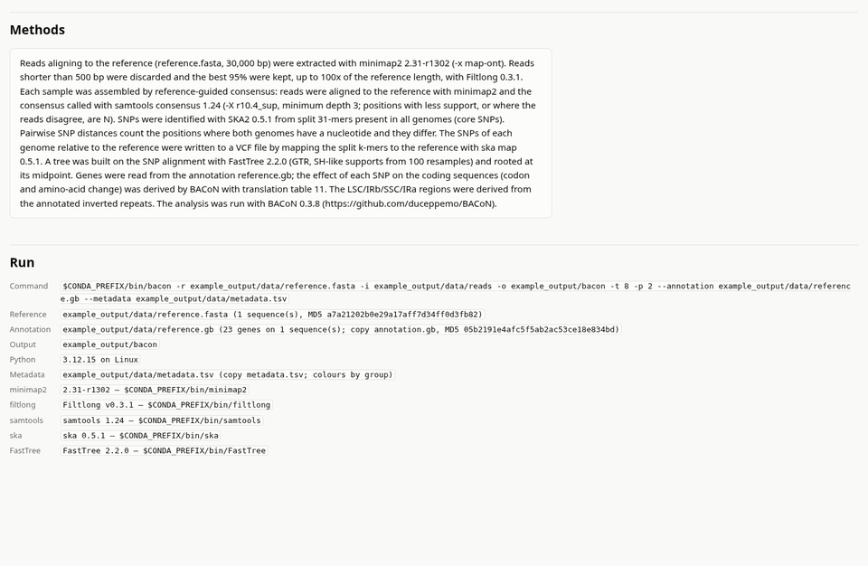
Methods and run. The methods paragraph describes what was run, with the program versions; the run section records the command, the reference's MD5, the annotation and metadata files and every program used.

Variations

Running the same command again with other options reruns only what changes (Usage):

• --color-by year colours the figures by year instead of group; --color-by none leaves them uncoloured (with or without --metadata); note is free text and cannot colour them. Nothing is redone, and the report is rebuilt. Without --metadata, the copy metadata.tsv that the first run wrote is removed.
• -r example_output/data/reference.gb without --annotation: the GenBank file is the reference and its own annotation; reference.fasta in the output folder is identical, so nothing is redone either.
• -a flye assembles de novo; --snp-method parsnp compares the assemblies with Parsnp instead of SKA2. Both give the same 20 SNPs and distances on this example (with Parsnp, 4_compared/parsnp/snps.vcf holds the same 20 records, and python example/check_example.py example_output parsnp passes the three checks).

For real data, see the Tutorial (28 potato cultivars) and its report.