Outputs

Outputs

OUTPUT/
├── report.html                 the report: samples, tree, distances, methods, provenance
├── summary.tsv                 one line per sample: reads, depth, assembly, status, notes
├── bacon_*_mqc.json            MultiQC sections (samples table, bases, SNP distances)
├── run_info.json               version, command, settings, program versions, samples, comparison
├── bacon.log                   the log of every run in this folder
├── .bacon.lock                 held by the run using this folder (see Usage)
├── reference.fasta             the reference used: upper case, ambiguity codes as N
├── annotation.gb / .gff3       the annotation of the reference (--annotation, or the GenBank reference), as given
├── metadata.tsv                the sample metadata (--metadata, and the sample sheet's extra columns), one row per sample and added genome
├── 1_extracted/<sample>.fastq.gz          baited reads (.fasta.gz for fasta input; <sample>.bam and .bam.bai
│                                          with --keep-bam)
├── 2_filtered/<sample>.fastq.gz           filtered reads (.fasta.gz for fasta input)
├── 3_assembled/
│   ├── all_assemblies/<sample>.fasta      the assembly of each sample
│   ├── assembly_graphs/<sample>.gfa/.png  assembly graphs (de novo assemblers; .png with Bandage)
│   └── <sample>/                          the assembler's own folder
├── 4_compared/
│   ├── added_genomes/<name>.fasta          genomes given with --add-genomes, as compared
│   └── <method>/                           ska, ska_<min-freq>, or parsnp
│       ├── snp_distances.tsv               pairwise SNP distances, Reference first
│       ├── tree.nwk                        midpoint-rooted tree (Newick)
│       ├── tree.svg                        picture of the tree
│       ├── snps.vcf                        SNPs of each genome relative to the reference (VCF)
│       ├── ska_reference.fasta             SKA2: the reference as used, extended when circular
│       └── ...                             the method's own files (alignments)
└── logs/<step>/<sample>.log              the commands run and the programs' messages

report.html

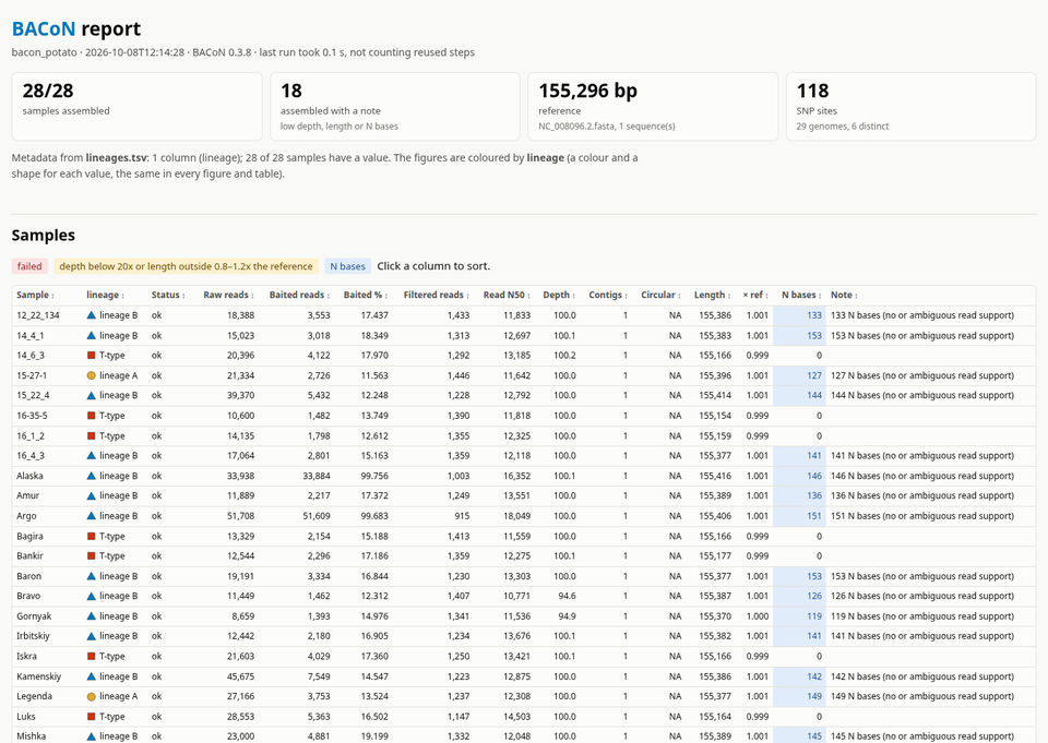
A self-contained web page (no internet connection needed) that opens in any browser and prints to PDF (the colours of the heatmap and of the highlighted cells are kept when printing):

• Overview: samples assembled, samples with a note, reference length, SNP sites and distinct genomes; with metadata, a line naming its source, its columns and the column that colours the figures.
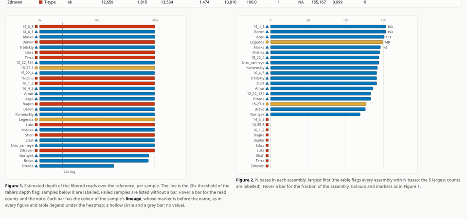
• Samples: the main columns of summary.tsv (all but the base counts, largest contig, assembly N50 and Flye's depth), sortable by clicking a header; failed samples, depth below 20x, length outside 0.8–1.2 times the reference, and N bases are highlighted. The metadata columns, when there are any, come right after Sample: a column whose values are all numbers sorts as numbers, long values wrap, the values of the colour column carry their marker (its colour and shape; a hollow circle alone when the sample has no value), and a column named like one of the table's own (Status, Note, Depth...) is headed Status (metadata). Without a colour column, the name of each genome in a group of identical genomes starts with the group's square. Two bar charts follow, sorted: the depth of each sample after filtering, with the 20x line (samples below it are labelled), and the N bases of each assembly (templated assemblies only: a de novo run gets a sentence instead of a chart of empty bars). Failed samples are listed without a bar. Each sample looks the same in the bar charts as everywhere else in the report: with a colour column, its bar has its value's colour (with the markers' thin dark edge) and its marker is drawn before its name, failed samples included (a grey bar and a hollow circle without a value); without one, its bar has the colour of its group of identical genomes, with the group's square before its name (a grey bar without a square for a genome in no group; groups beyond the 12th are grey, with a square); without a comparison either, the bars keep their single blue. The legend of the colour column is the heatmap's; when there is no heatmap (no comparison, more than 150 genomes), or a value is held by failed samples only, a line under the bar charts gives each value's marker and number of samples. The groups' legend is the list of identical genomes.
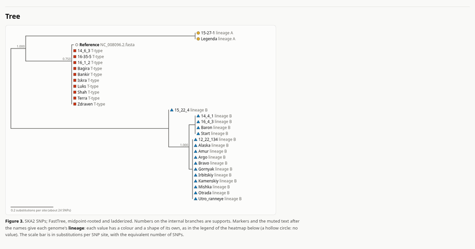
• Tree: drawn from tree.nwk, midpoint-rooted and ladderized, with the supports on the internal branches, a scale bar (with its equivalent number of SNPs for SKA2), and a coloured square with a thin dark edge for each group of identical genomes (12 colours, then grey); or why there is none. With a colour column, colour is given to the column only: each leaf gets the marker of its value, a colour and a shape (a hollow circle when the genome has none, as the reference), and the value in muted text after the name, instead of the group square. Each value has a marker of its own, up to 48 values (12 colours from the colourblind-safe palettes of Okabe & Ito and of Paul Tol, and seven shapes: circle, triangle, square, diamond, inverted triangle, plus, cross). Up to 25 values, two values whose colours look alike to a colourblind reader differ by their shape; with more, a few pairs sharing a shape may look alike, and the legend and the value after each name tell them apart (Usage). The light and dark themes and the printed page keep the markers, but with many genomes the printed tree and heatmap are shrunk to fit the page, and the markers with them (at 150 genomes the heatmap's are under a millimetre across).
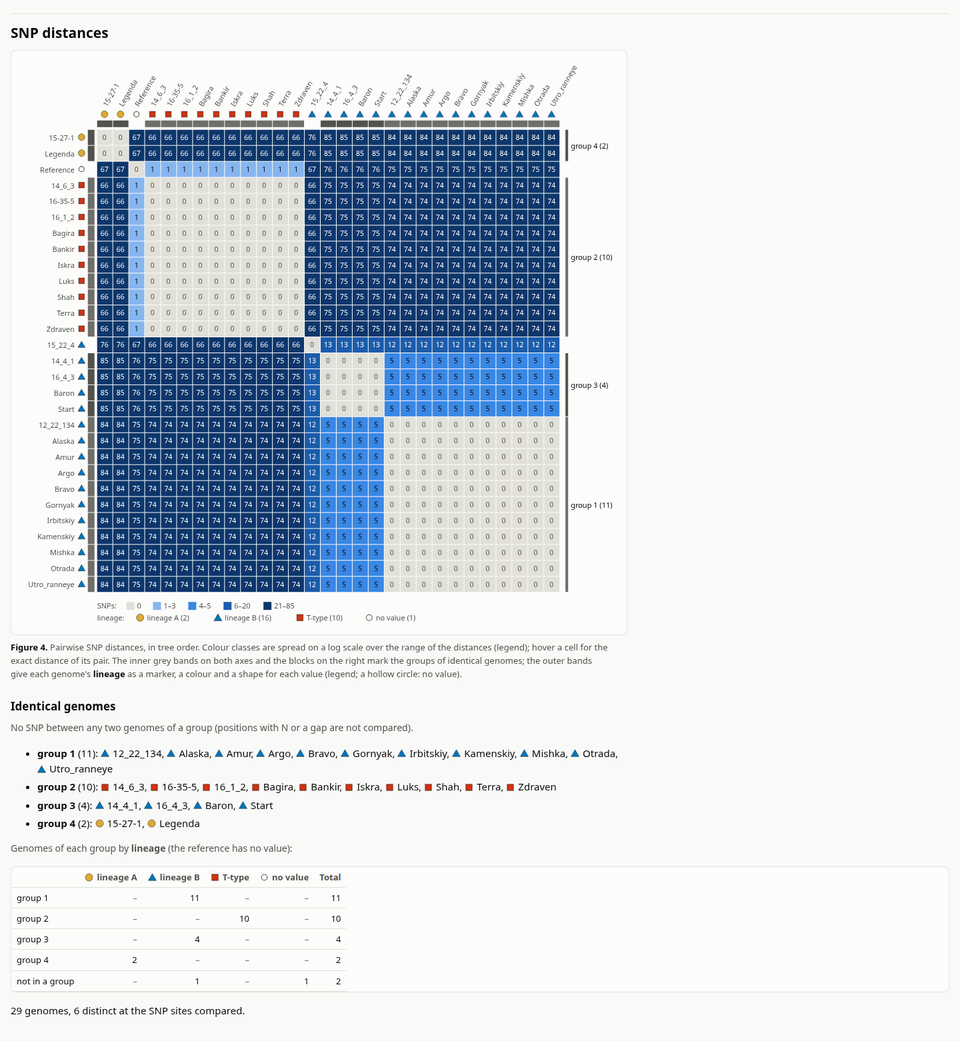
• SNP distances: a heatmap in the order of the tree, with colour classes spread over the range of the distances (so that 1–5 SNP differences stay visible next to larger ones) and the exact distance on hover. The groups of identical genomes, with no SNP between any two members, are coloured bands along both axes and labelled on the right, and are listed below with the number of distinct genomes (positions with N or a gap are not compared, so a genome with missing data could match two genomes that differ: it is put in one group only). With a colour column, a second band outside the first gives each genome's marker (a hollow circle when it has none), with its own legend of markers, values and counts (on rows of their own, headed by the column's name, under the row of distance classes headed SNPs:), and the list of identical genomes is followed by a table counting the genomes of each group (and those in no group) for each value, with the values' markers (each genome of the list also has its marker before its name) (as columns, or as rows above 12 values when there are more values than groups, so that the table fits a printed page). The groups of identical genomes are then drawn in two alternating greys, so that colour means the column's values only. Without any SNP site, no identity is claimed. Above 150 genomes the heatmap is left out (the distances are in snp_distances.tsv).
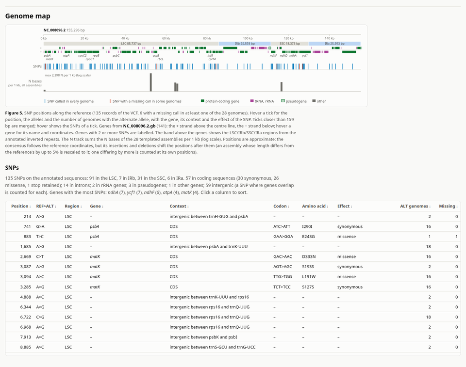
• Genome map: each reference sequence with the positions of the SNPs of snps.vcf (the records that passed their filters: Parsnp's filtered SNPs are not in the distances, and the caption counts them), coloured by whether every genome has a call there (blue) or some genome has none (red); for templated assemblies (whose coordinates follow the reference), the N bases per kb (coarser bins above 1.5 Mb) summed over the assemblies of the run's samples, at approximate positions: the insertions and deletions of a consensus shift the positions after them, so an assembly whose length differs from the reference's by up to 5% is rescaled to it (one differing by more is a partial consensus, counted at its own positions). A band of the plastome regions (LSC, IRb, SSC, IRa), with or without an annotation: from the annotation's two inverted repeats of at least 500 bp (named as the annotation names them, otherwise by convention: the larger single-copy region is the LSC and the repeat after it IRb; the single-copy regions are the gaps between the repeats, one of which may span the origin), or else from the large inverted repeat detected in the reference sequence itself (two copies of at least 5 kb, at least 99% identical, in a sequence of 2 Mb or less), when the regions have the layout of a plastome (the repeats at least 5% of the sequence, the larger single-copy region at most 200 kb, the record not said to be a mitochondrion or a chromosome: Methods); the caption says which, with the detected copies' size and identity, and where the band is for each sequence (above the genes, or under the axis for a sequence without annotation), and the hover of a SNP on a sequence without annotation gives its region. With an annotation (--annotation, or a GenBank reference), the map also shows: the genes of the + strand above a centre line and those of the − strand below (protein-coding genes in green, tRNA and rRNA genes in purple, pseudogenes as a faint green fill with a green outline, other genes in grey), each with its name, type and coordinates on hover; labels for the genes with two or more SNPs (at most 40, those with the most SNPs, on two rows; a gene without a symbol is labelled by its product when that is at most 12 characters, tRNA-Val, else by its locus tag, LK299_pgr007); and, on each SNP's hover, its gene, context and effect. Above 1,500 genes (a bacterial genome), the gene rows only show where genes lie, merged per pixel, without names or labels.
• SNPs (with an annotation): a summary (SNPs per region, per context and by effect, the genes with the most SNPs, and the SNPs on sequences without annotation, if any) and a sortable table with one row per SNP of the VCF: the sequence (when the reference has several), position, alleles, region (also for a sequence without annotation, from its band; the summary counts those too), gene (its symbol, or locus_tag (product) for a gene without one, such as LK299_pgr007 (23S ribosomal RNA)), context (CDS, intron, tRNA, rRNA, pseudogene, UTR, or intergenic between X and Y, the nearest genes on either side, around the origin of a circular sequence), the codon and amino-acid change and the effect (synonymous, missense, nonsense, stop lost, stop retained (a stop codon changed into another), start lost, start retained: a changed start codon that is still one in the genetic code used), and the number of genomes with the alternate allele or without a call. A SNP in several alternate alleles, or in two overlapping coding sequences, has one effect per allele and per gene. A summary line gives the SNPs per region and per context, the counts of each effect and the genes with the most SNPs. The table shows at most 3,000 SNPs (by position). How the effects are computed is in Methods.
• Methods: a paragraph describing what was run, with program versions (and the annotation, when the map drew its genes, with the translation table when SNPs were annotated with it, and, when the report shows the LSC/IRb/SSC/IRa band, where the regions come from: the annotated inverted repeats, or the one detected in the reference sequence, with the copies' size and identity), ready to adapt for a paper.
• Run: command, reference (with the MD5 of the file as given), the annotation when there is one (the file as given, --annotation or the GenBank reference, with its MD5 and BACoN's copy), output folder, the metadata file and the colour column when there are any (not applied when the folder's metadata.tsv was edited since and can no longer colour the figures; a note says why), and the version and path of every program.

It is written at the end of every run, from the files of the output folder; python -m bacon.report OUTPUT rebuilds it, also after the folder was moved. Examples: the bundled example and the tutorial.

MultiQC

Three MultiQC custom-content files, found automatically by multiqc in the output folder or any folder above it:

File	MultiQC section
bacon_samples_mqc.json	table: the metadata columns (as text), status, baited reads and share, read N50, depth, contigs, circular contigs, length, length vs reference, N bases, note
bacon_reads_mqc.json	bar graph: the bases of each sample kept for the assembly, baited but filtered out, and off-target
bacon_distances_mqc.json	heatmap of the SNP distances in tree order (recent MultiQC versions also offer a clustered view); absent when the samples were not compared

multiqc OUTPUT/ --ignore "*/logs/*"

• The sections are named after the output folder ("BACoN folder: samples"), so the files of several BACoN runs in one MultiQC search path give separate sections, as long as the output folders have different names. The section ids keep a name of letters, digits and underscores as it is; any other name gets a short hash of itself, so that names differing only in punctuation (run-1, run_1, run 1) do not merge.
• --ignore "*/logs/*" keeps MultiQC away from the programs' logs in logs/: MultiQC 1.19 mistakes BACoN's Filtlong logs for its own module's input and shows an error box (harmless; 1.35 does not).
• MultiQC shortens sample names ending with usual file suffixes (such as .trimmed) in the table and bar graph, but not in the heatmap.
• The heatmap's distances are whole numbers in recent MultiQC versions (1.35); older versions such as 1.19 ignore the setting and show them with two decimals (10.00).

Tested with MultiQC 1.19 and 1.35.

summary.tsv

Column	Description
Sample	Sample name
Status	ok, or failed (step) with the reason in Note
Raw_reads, Raw_bases	Input reads and bases (NA with -b bbduk when BBDuk does not report them)
Baited_reads, Baited_bases, Baited_pct	Reads matching the reference, and their share of the input bases (%)
Filtered_reads, Filtered_bases, Filtered_N50	Reads kept by Filtlong (fasta reads: by BACoN's length filter, --min-read-length)
Est_depth	Filtered bases / genome size (-s, or the reference length)
Contigs	Number of contigs
Circular_contigs	Contigs the assembler reports as circular (Flye, myloasm; NA for the templated assembly)
Assembly_length, Largest_contig, Assembly_N50	Assembly statistics
Length_vs_reference	Assembly length / reference length
Assembly_depth	Mean depth reported by Flye
N_bases	Templated assembly: bases called N, where fewer than three reads cover the reference or the reads disagree (often inside insertions)
Note	Warnings: low depth (below 20x), assembly length outside 0.8–1.2 times the reference, N bases, or why the sample failed

Assemblies

3_assembled/all_assemblies/<sample>.fasta holds one sequence per contig, named <sample>_<contig>. Contigs that the assembler reports as circular have circular=true in their header.

• Templated (samtools): one sequence per reference sequence, in reference coordinates plus the sample's insertions and minus its deletions. Positions covered by fewer than three reads, and bases the reads do not agree on (often inside an insertion), are N.
• De novo (flye, myloasm): contigs as assembled. A circular genome can start anywhere and on either strand. Chloroplasts often come out as three contigs (large single copy, inverted repeat, small single copy) when the reads are shorter than the inverted repeat.

Comparison

snp_distances.tsv is a square matrix of the number of positions where two genomes have different nucleotides (A, C, G, T; gaps and N are ignored), with the reference as Reference.

• SKA2 (4_compared/ska/, or ska_<min-freq>/): ska.snps.fasta is the alignment of the SNP sites (the columns with at least two different nucleotides). A SNP in an inverted repeat is counted once (its two copies share the same split k-mer).
• Parsnp (4_compared/parsnp/): parsnp.core.fasta is the core-genome alignment, used for the tree; parsnp.snps.fasta the SNP sites; plus Parsnp's own files.

snps.vcf lists, for each position of the reference where a genome has a SNP, the genotype of every genome: 1 (or 2, 3 at a position with several alternate alleles) for an alternate allele, 0 for the reference allele, . when the genome lacks the position or its base there is ambiguous. There is one column per genome, sorted by name; the reference itself has no column. Contig names and lengths are those of the reference. On the simulated plastid of the validation (both methods, templated and de novo assemblies), the files load in bcftools without warnings, their reference alleles match the reference (bcftools norm --check-ref), and SKA2's hold exactly the SNPs of the truth.

• SKA2: from ska map, which maps the split k-mers of every genome to the reference as SKA2 used it (extended by the start of each sequence when more than half of the samples' assemblies have a circular contig, so that SNPs next to the ends are kept; ska_reference.fasta in the comparison folder; see Methods). All SNPs are listed, whatever --ska-min-freq (which only affects the alignment, the distances and the tree). A SNP in both copies of an inverted repeat is listed at both of its positions; a difference between the two copies of one genome is ambiguous and is not listed.
• Parsnp: from HarvestTools: the SNPs of the core-genome alignment, with Parsnp's filters in the FILTER column: PASS, or the reasons a SNP was left out of the alignment, and so of the distances and the tree (ALN, CID, LCB, IND, N, several joined by :; see Methods). The report shows the PASS records only, and says how many others the file has. SNPs in inverted repeats are missing, as in the distances, and so are SNPs within about 30 bases of the ends of the reference (SKA2, with templated assemblies: within 15 bases).

N is never an allele: a genome's N gives .. Positions where no genome has an alternate allele (a deletion, missing data) are left out, and so are positions where the reference's own sequence is ambiguous (its split k-mer occurs with different middle bases, in repeats).

tree.nwk is rooted at the midpoint of the longest path and ladderized; internal labels are the supports (SH-like local supports from 100 resamples for FastTree, ultrafast bootstraps for IQ-TREE). tree.svg draws it with a scale in substitutions per site. When no SNP site is shared by all the genomes, the distances are written but no tree is built; lower --ska-min-freq (see FAQ), unless the genomes do not differ at all (an empty VCF; the report says so).

run_info.json

The provenance of the last run: BACoN version, command line, start time and duration, all settings, the path and version of every program used, the reference as given (path, number of sequences, length and the MD5 of the file itself, fasta or GenBank, and for each of its sequences the LSC/IRb/SSC/IRa regions with their source, annotation or sequence, and for the latter the detected copies' coordinates, lengths, differences and identity, or "none"; an inverted repeat that is not a plastome layout, the repeat of a mitochondrion or the inverted rRNA operons of a bacterium, is recorded with "source": "none", no regions and a note saying why), the annotation when there is one (file, format, the name of its copy in the output folder, numbers of genes and of annotated sequences, whether regions were derived, the translation tables, MD5), the sample metadata when there is some (the --metadata file and its MD5, the sample sheet's metadata columns, the name of the copy, the columns, how many samples have a row, how many rows match no sample, and the colour column, null when none), each sample's files and status, and the comparison's result files.