Examples gallery
Every example below ships as a runnable script in
examples/.
The output PNGs are committed under
docs/images/
and the canonical paletted GeoTIFFs alongside them — drop the TIFF
into QGIS to see the color table and class names attached as
metadata.
The three workflows complement each other:
| Scale | Input | Samples / pixels | Example |
|---|---|---|---|
| Regional | Gridded rasters (SoilGrids) | 740,745 pixels | soilgrids_france.py |
| Synthetic field | Sparse samples + simple polygon | 20 samples on 100 m × 100 m | field_kriging.py |
| Minimal field survey | Sparse samples + irregular polygon | 3 samples on a 10 ha plot | central_france_field.py |
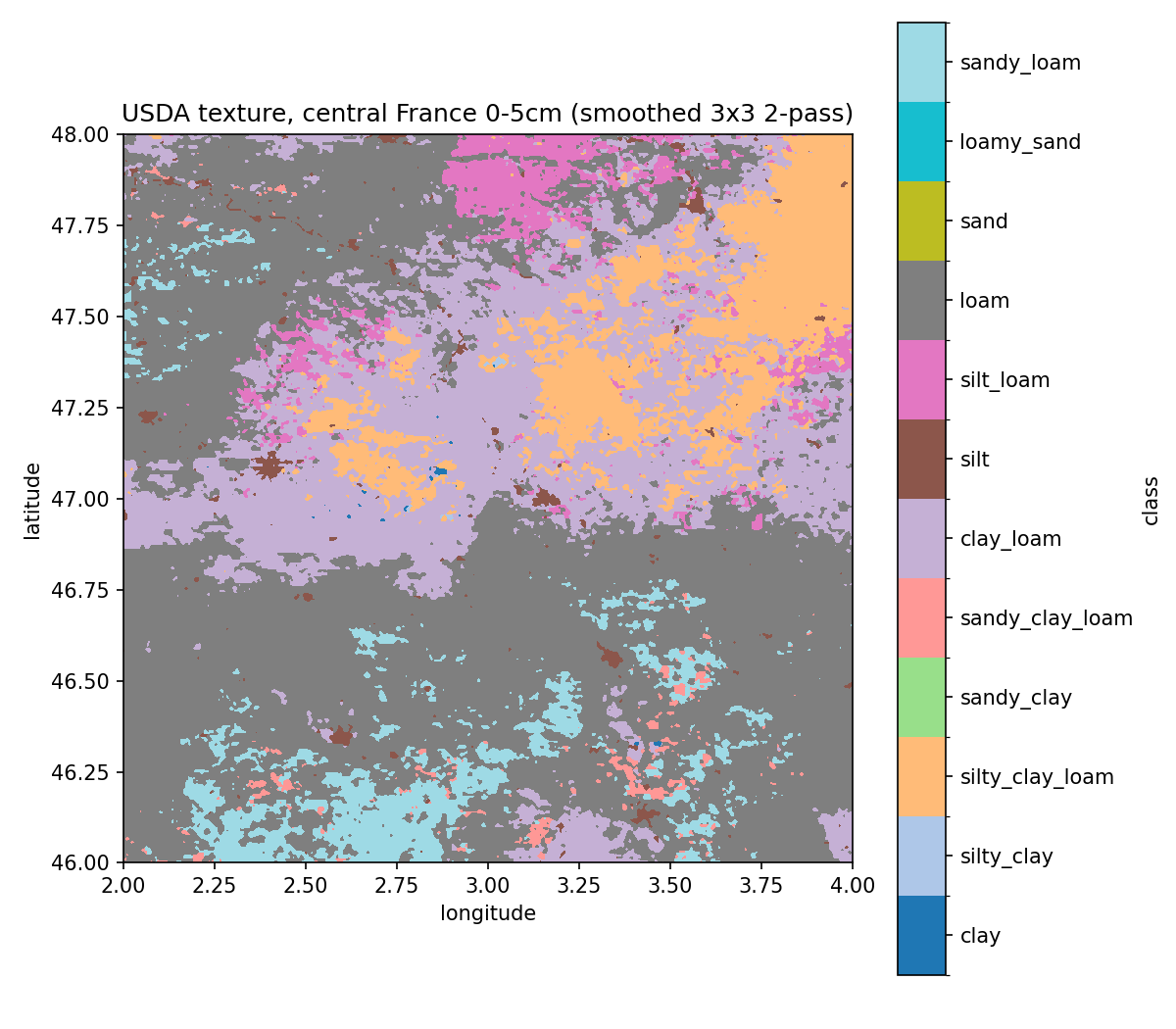
What you're seeing. A 2°×2° tile (lon 2°-4°E, lat 46°-48°N, approximately the Allier / Cher / Nièvre region) of the ISRIC SoilGrids 2.0 dataset, sand and clay fractions at 0-5 cm depth, classified pixel-by-pixel under USDA. 740,745 pixels at the native ~250 m resolution. The raw classification is post-processed with a 3×3 majority filter (2 passes) to remove salt-and-pepper noise between adjacent classes.
Workflow.
SoilGrids WCS (sand + clay GeoTIFFs)
  → classify_geotiff (USDA, units="g/kg")
  → smooth_codes (3×3 majority, 2 iterations)
  → write_classified_geotiff (paletted uint8)
  → render_classified_png (matplotlib + side legend)
Numbers (Apple M-series, repo at HEAD).
| Step | Time |
|---|---|
| Classify 740,745 pixels (USDA) | ~0.12 s |
| 2 majority-smoothing passes | ~0.3 s |
| Polygonize → Shapefile | ~0.3 s |
| Total end-to-end (download cached) | ~1.5 s |
Run it.
pip install 'pedotri[raster,matplotlib]'
python examples/soilgrids_france.py
First run downloads the three SoilGrids tiles via the ISRIC WCS
endpoint and caches them under
tests/data/soilgrids_france/.
Files.
- Script:
examples/soilgrids_france.py - PNG:
docs/images/usda_central_france.png - TIFF:
docs/images/usda_central_france.tif(paletted uint8, 50 KB)

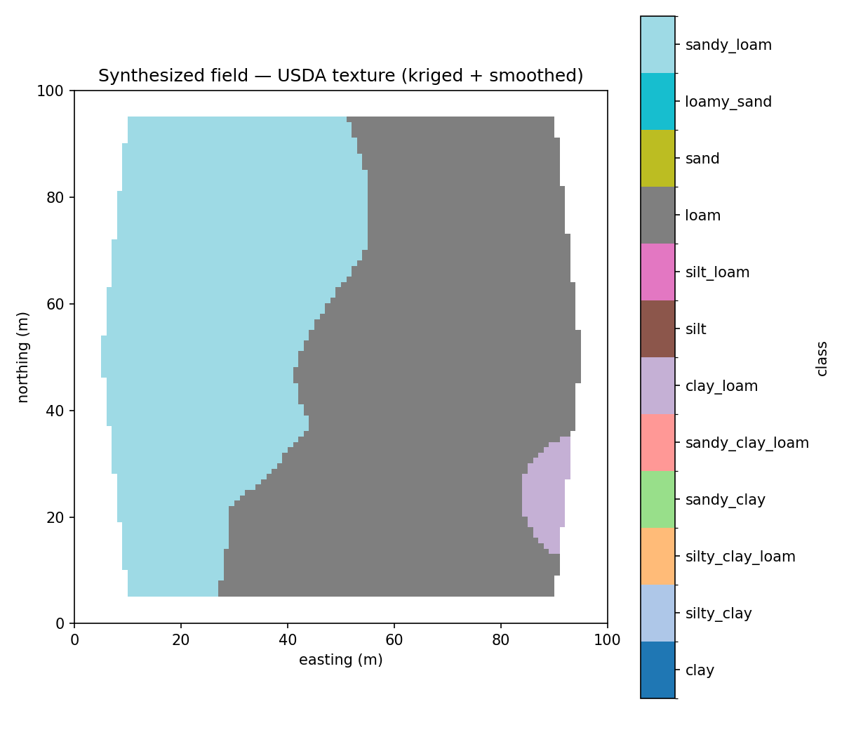
What you're seeing. A purely synthetic 100 m × 100 m hexagonal plot with 20 in-situ samples placed at random inside the boundary. The samples are drawn from a deliberate SE→NW gradient (sand % increasing toward the NW). Ordinary kriging interpolates the samples onto a 1 m grid; cells outside the hexagon are masked.
This example shows the "well-sampled" end of the field-survey spectrum — enough samples that the variogram fits cleanly and the result is a believable continuous map.
Workflow.
samples + hexagonal boundary
  → krige_sand_clay (variogram="spherical", mask_polygon=boundary)
  → classify_array (USDA)
  → smooth_codes
  → write_classified_geotiff + render_classified_png + write_features_shapefile
Run it.
pip install 'pedotri[raster,vector,interp,matplotlib]'
python examples/field_kriging.py
Files.
- Script:
examples/field_kriging.py - PNG:
docs/images/field_usda.png - TIFF:
docs/images/field_usda.tif

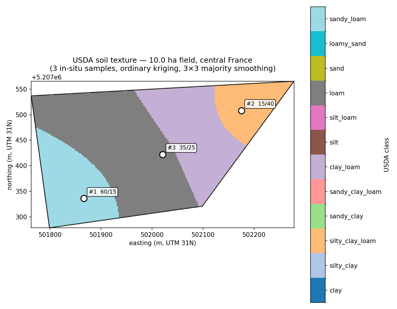
What you're seeing. A pseudo-random 10 ha field generated from a fixed seed (so it's fully reproducible) inside the same central- France bounding box as the SoilGrids regional example above — specifically around 47°N, 3°E. The field polygon is the convex hull of 7 random points, rescaled to exactly 10 hectares; coordinates are EPSG:32631 (UTM zone 31N, metres).
Three soil samples are placed in distinct sub-areas: a sandy_loam spot in the SW (sand 60 % / clay 15 %), a silty_clay spot in the NE (15 % / 40 %), and a loam spot near the centre (35 % / 25 %). Ordinary kriging with a linear variogram interpolates them onto a 2 m grid masked to the field boundary; the result is classified as USDA texture, smoothed 3×3, and rendered with the sample markers overlaid.
Why three samples is the minimum. pyKrige's variogram fitter
needs at least three pairwise distances, so n = 3 is the absolute
floor for ordinary kriging. With so few points, only the linear
variogram model fits reliably (the spherical/exponential/gaussian
models all have too many free parameters for three observations).
The example uses variogram="linear" and n_lags=2 accordingly.
The resulting map has four visible USDA classes: a sandy_loam wedge
in the SW, a loam middle band, a clay_loam zone, and a silty_clay_
loam patch around the NE sample. Don't read too much into the
exact boundaries — between samples the map is essentially a
linear interpolation. For production work, aim for 8-15 samples
per field and check the per-cell kriging variance returned by
krige_samples as a confidence map.
Workflow.
random_field_polygon(target_ha=10, seed=2024)
sample_layout(field)  # 3 samples in different quadrants
  → krige_sand_clay (variogram="linear", n_lags=2, mask_polygon=field)
  → classify_array (USDA) → smooth_codes (3×3, 2 passes)
  → write_classified_geotiff + render with sample markers overlaid
Run it.
pip install 'pedotri[raster,vector,interp,matplotlib]'
python examples/central_france_field.py
Files.
- Script:
examples/central_france_field.py - PNG:
docs/images/central_france_field.png - TIFF:
docs/images/central_france_field.tif

Not pictured (text-only output) but worth flagging:
examples/bench_soiltexture.py
runs the head-to-head benchmark against the soiltexture
Python package. On USDA, 740,745 points: pedotri ≈ 6.3 M pts/sec,
soiltexture ≈ 130 k pts/sec → 48× speedup, 100 % output
agreement. See Benchmark-vs-soiltexture
for the writeup.
pip install pedotri soiltexture
python examples/bench_soiltexture.py- Map-products-and-field-sampling — the same two workflows with prose walkthroughs and API details
- GeoTIFF-and-SoilGrids — SoilGrids download / preprocessing specifics
- Benchmark-vs-soiltexture — performance writeup