Uncertainty aware classification
Modern digital soil maps don't ship a single number per property — they ship a distribution. SoilGrids, for instance, publishes Q0.05 / Q0.50 / Q0.95 quantile layers alongside the mean for clay, sand, silt, SOC, bulk density, and friends. Classifying the mean and walking away throws that information out at the most expensive moment: right before you make a decision.
Pedotri 0.3 makes uncertainty a first-class citizen of pedotri.classify.
A point at (sand=27 %, clay=45 %) sits inside USDA clay when you classify the mean. Stretch its 90 % CIs to ±10 % on each axis and roughly 23 % of the distribution's mass spills into neighbouring classes — clay loam, silty clay loam, silty clay. The honest answer isn't a single label; it's a distribution over classes, and how peaked that distribution is tells you how much weight to put on the modal answer.
Pedotri offers two ways to summarize this.
When you pass uncertainty kwargs, the default method="distance" looks at
the signed distance between your point and its class boundary, compares it
to the input uncertainty, and returns a single confidence number in
[0, 1]:
import pedotri
from pedotri.uncertainty import Quantiles

r = pedotri.classify(
    sand=27, clay=45,
    sand_uncertainty=Quantiles(20, 34),     # Q0.05 / Q0.95
    clay_uncertainty=Quantiles(38, 52),
    classification="USDA",
)
r.key         # 'clay'
r.distance    # 5.0      — units of the (sand %, clay %) plane
r.confidence  # 0.88     — Φ(distance / σ_effective)
Passing any *_uncertainty kwarg automatically promotes the return
type to ClassifyResult — you don't need to spell out detailed=True
explicitly. For backwards compatibility a bare (q05, q95) 2-tuple is
still accepted but emits a DeprecationWarning; wrap it in
Quantiles to silence the warning and make the call site
self-documenting. sand_uncertainty= also accepts a plain scalar or
array — interpreted as σ directly — for when you've already fit a
distribution and want to pass the spread without re-deriving it from
quantiles.
Under the hood, σ for each axis is derived from the Q05/Q95 pair, combined into an isotropic σ_effective (quadratic mean across axes), and fed into the standard normal CDF. A point sitting many σ inside its class scores near 1.0; one sitting right on a boundary scores 0.5.
This costs essentially the same as a normal classification — one extra
distance computation and one erf call — so it's cheap enough to be the
default whenever uncertainty kwargs are supplied. What it doesn't give
you is a probability distribution over neighbouring classes. For that,
sample.
method="monte_carlo" draws n_samples realizations from your input
distribution, classifies each, and tallies a full probability table:
r = pedotri.classify(
    sand=27, clay=45,
    sand_uncertainty=Quantiles(20, 34),
    clay_uncertainty=Quantiles(38, 52),
    classification="USDA",
    method="monte_carlo",
    n_samples=1000,
    seed=42,
)
r.key                          # 'clay'    — modal class
r.probabilities                # {'clay': 0.842, 'clay_loam': 0.138, ...}
r.entropy                      # 0.51 nats — how spread the distribution is
r.confidence                   # 0.842     — modal-class probability
r.unclassified_probability     # 0.0       — fraction outside any class
entropy is reported in nats; its maximum is log(n_classes), hit when
every class is equally likely.
Sand, silt and clay are constrained to sum to 100 %. Independent normal
samples per axis can produce invalid compositions where sand + clay > 100.
Pedotri's sampler handles this by projecting offending draws onto the
nearest edge of the simplex (silt → 0, sand and clay scaled down
proportionally to preserve their ratio). The output is therefore always
a valid texture composition.
For 1-D classifications such as KACHINSKY, there is no compositional
constraint; the single axis is sampled as a clipped truncated normal on
[0, 100].
Pass seed= (any int or numpy.random.Generator) for deterministic
sampling. Without a seed, each call draws fresh randomness.
| If you want… | Use |
|---|---|
| A confidence score on the modal class, fast |
method="distance" (default) |
| The full probability distribution over classes | method="monte_carlo" |
| Entropy as a "how messy is this pixel" indicator | method="monte_carlo" |
| To run uncertainty over a raster of millions of pixels |
method="distance" for the default pass, MC only on flagged pixels |
The distance method is roughly 100×–1000× cheaper than Monte Carlo with
n_samples=1000, depending on classification complexity. At raster scale
that gap matters a lot.
Two assumptions worth being explicit about, because they affect how you should read the output:
-
Distribution shape. When you pass
(Q05, Q95), pedotri fits a normal clipped to[0, 100]. The Q05/Q95 pair doesn't uniquely determine a distribution; this is the standard truncated-normal assumption used in most soil texture uncertainty work. For strongly skewed properties (SOC, hydraulic conductivity), a log-normal fit would be more faithful. Not yet supported — pass a pre-computed σ if you've already fit a different shape. -
Spatial autocorrelation. When you run Monte Carlo over a raster (coming in 0.3.x via
zonal_aggregate), pedotri treats each pixel as an independent draw. SoilGrids residuals are highly spatially correlated; an independent-pixel assumption underestimates the uncertainty of regional averages. The 0.4 roadmap covers correlation-aware sampling. For 0.3, treat aggregated MC uncertainty as a lower bound.
import pedotri
from pedotri.uncertainty import Quantiles

base = dict(sand=27, clay=45, classification="USDA",
            method="monte_carlo", n_samples=2000, seed=0)

for width in (2, 5, 10, 20):
    r = pedotri.classify(
        **base,
        sand_uncertainty=Quantiles(27 - width, 27 + width),
        clay_uncertainty=Quantiles(45 - width, 45 + width),
    )
    top = sorted(r.probabilities.items(), key=lambda kv: -kv[1])[:3]
    print(f"±{width}%:  entropy={r.entropy:.3f}  top3={top}")
±2%: entropy=0.000 top3=[('clay', 1.0)]
±5%: entropy=0.215 top3=[('clay', 0.949), ('clay_loam', 0.048), ('silty_clay', 0.002)]
±10%: entropy=0.706 top3=[('clay', 0.770), ('clay_loam', 0.176), ('silty_clay_loam', 0.032)]
±20%: entropy=1.438 top3=[('clay', 0.548), ('clay_loam', 0.185), ('silty_clay_loam', 0.086)]
You can read this as: the same point classifies with full confidence under tight CIs and bleeds into neighbouring classes as the input CI widens. Uncertainty isn't optional context — it's the answer.
Two implementation choices show up in profiles and are worth being explicit about — both trade a tiny, well-quantified amount of numerical fidelity for a 3–5× speedup and, crucially, a zero-extra-dependency core install.
The distance method converts a signed distance-to-boundary, expressed
in σ units, into a confidence number via the standard-normal CDF
Φ(k) = ½(1 + erf(k / √2)). The shape of erf here is just the
"area under a Gaussian": a pixel sitting 0 σ from the boundary scores
0.5, one sitting 1 σ in scores 0.84, 2 σ in scores 0.977, and so on.
The catch is that the Python stdlib's math.erf is a scalar function.
On a 1 Mpix SoilGrids tile passed through
classify_array_with_uncertainty(..., method="distance") we call erf
a million times per call. Three implementations:
| Implementation | Time on 1 Mpix | Dependency |
|---|---|---|
np.vectorize(math.erf) — Python per cell |
~60 ms | none |
| Abramowitz & Stegun 7.1.26 in pure numpy | ~13 ms | none |
scipy.special.erf |
~11 ms | scipy |
pedotri ships with the middle option. The coefficients come verbatim
from formula 7.1.26 of Milton Abramowitz and Irene Stegun's Handbook
of Mathematical Functions (1965), a standard reference for
numerical-method polynomial approximations. The formula is a
five-term polynomial in t = 1 / (1 + 0.3275911 · |x|) multiplied by
exp(−x²), and is documented to give a maximum absolute error
ε ≤ 1.5 × 10⁻⁷ across the entire real line — well below the
precision we report to users (confidence values surface with
three significant figures, and float32 itself only has ~seven).
We get the 5× speedup without dragging scipy into the core install;
scipy stays optional under the [raster] extra for users who want
its other goodies.
This affects every distance-method call:
-
pedotri.classify(..., method="distance")— single-point and array. -
pedotri.raster.classify_array_with_uncertainty(..., method="distance")— produces theconfidenceraster you can render or write as a GeoTIFF.
The Monte-Carlo paths don't touch erf at all (they tally class hits
instead) — so the speedup is exclusive to the distance method.
Every Monte-Carlo path in pedotri (1-axis classify, the simplex
sampler sample_compositional, the regional sampler in
zonal_aggregate) draws values from a normal distribution and pins
out-of-range draws to the support boundary [0, 100].
The textbook alternative — scipy.stats.truncnorm — instead rejects
out-of-range draws and redraws them, producing a distribution with
exactly zero mass outside the support. The difference matters when
σ is large relative to the distance from the support boundary; it
doesn't matter when σ is small.
Concrete numbers for soil texture:
- SoilGrids σ on sand fractions is typically 3–7 percentage points,
while the support is the full
[0, 100]interval (97 percentage points wide). - For a pixel with mean = 27 %, σ = 5 %, the fraction of draws that
would need clipping is roughly
Φ(−27/5) ≈ 6 × 10⁻⁸. Negligible. - The pathological case is mean very close to 0 or 100. At mean = 1 %, σ = 10 %, about 16 % of draws get clipped to 0; this introduces a real bias toward the boundary. We document this and don't fix it in core, because the bias is still smaller than the spatial-autocorrelation lower bound we already disclose for regional aggregates.
If your inputs do sit near the boundary and you need the rigorous
truncated-normal samples, you can sample upstream with
scipy.stats.truncnorm.rvs and feed the σ array into
zonal_aggregate via the "sigma" property-spec form — pedotri will
use your values as-is and only clip on its own internal redraws if
they overshoot.
Three cases:
-
No uncertainty supplied.
r.confidence is None— the deterministic modal class is the answer. -
Distance method, point unclassified.
r.key is Noneandr.confidence is nan(round-tripped toNoneinto_dict). -
Distance method, zero σ on every axis.
r.confidence is nan. This is a degenerate input — if you passsand_uncertainty=Quantiles(50, 50), the distribution has zero spread, so there's no probabilistic content to summarize. Drop the kwarg in that case.
The same primitives work pixel-wise through
pedotri.raster.classify_array_with_uncertainty and
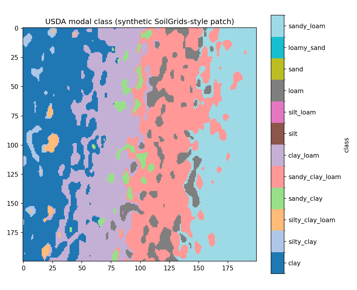
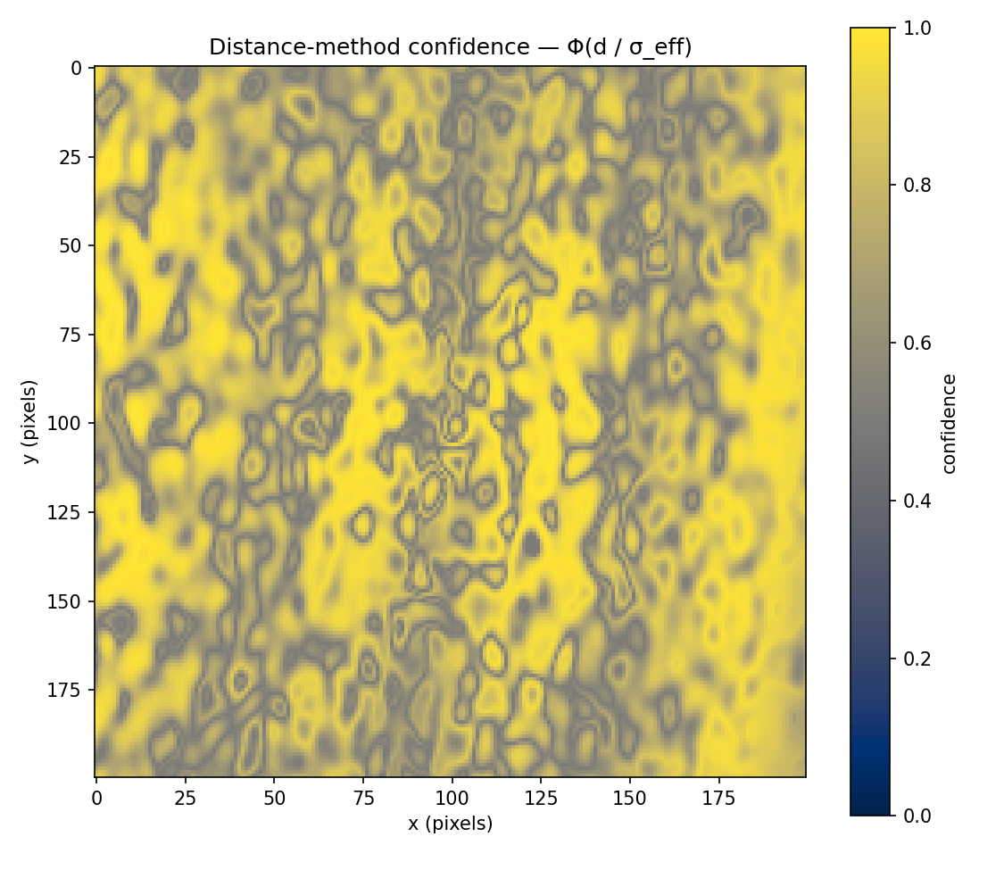
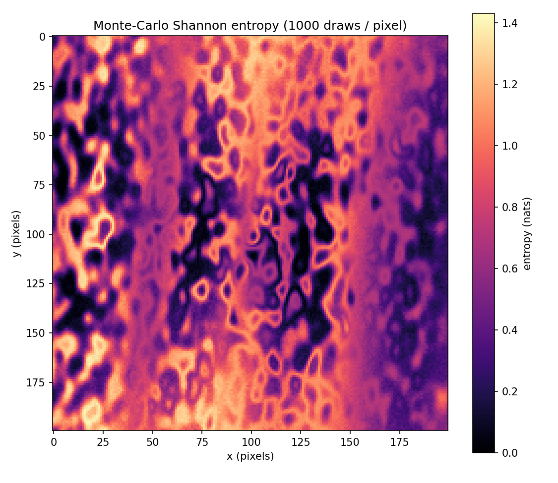
classify_geotiff_with_uncertainty. The maps below come from a
synthetic 200×200 patch where sand grades left-to-right, clay
counter-grades, and uncertainty (σ) rises from the center toward the
edges — so confidence and entropy structure don't just trace class
boundaries.
Modal class. The deterministic classification of the mean: nine USDA classes appear across the gradient.
Distance-method confidence. Φ(distance / σ_eff). Bright pixels
sit deep inside a class with σ small relative to boundary distance;
dark pixels straddle a boundary or live where σ is large.
Monte-Carlo entropy. Shannon entropy of the per-pixel class distribution, 1000 draws per pixel. Bright pixels are ambiguous in the distributional sense — neighbouring classes have substantial mass — and reliably outline the same boundary regions the confidence map flags. Entropy adds information confidence alone doesn't: a pixel that splits two-ways looks different from one that splits four-ways.
The Monte-Carlo path also writes a top-5 probability GeoTIFF with
ten bands: five class-code bands (rank_1_class … rank_5_class,
uint8 with 255 as nodata) and five probability bands
(rank_1_prob_x255 … rank_5_prob_x255, uint8 scaled
0–255). Dataset-level tags carry the class-key mapping
(class_0 … class_n-1) and the active top_k value, so the
file is self-describing without external metadata. Reproduce all of
the above with::
python examples/uncertainty_demo.py
- GeoTIFF and SoilGrids — how to wire SoilGrids rasters into the classifier (uncertainty bands coming in 0.3.x).
- Classification challenges — why boundary-adjacent pixels are inherently messy and what the literature has tried.