Tutorial Annotations
Prerequisites: Viewer loaded with a dataset
Time required: ~10–20 minutes
Tissue annotations let you label regions of the slide with named types such as tumour, stroma, or vessel. Annotated regions are used in the Annotation Neighbourhood and Annotation Distance tabs for spatial analysis, and can be exported as GeoJSON for use in other tools.
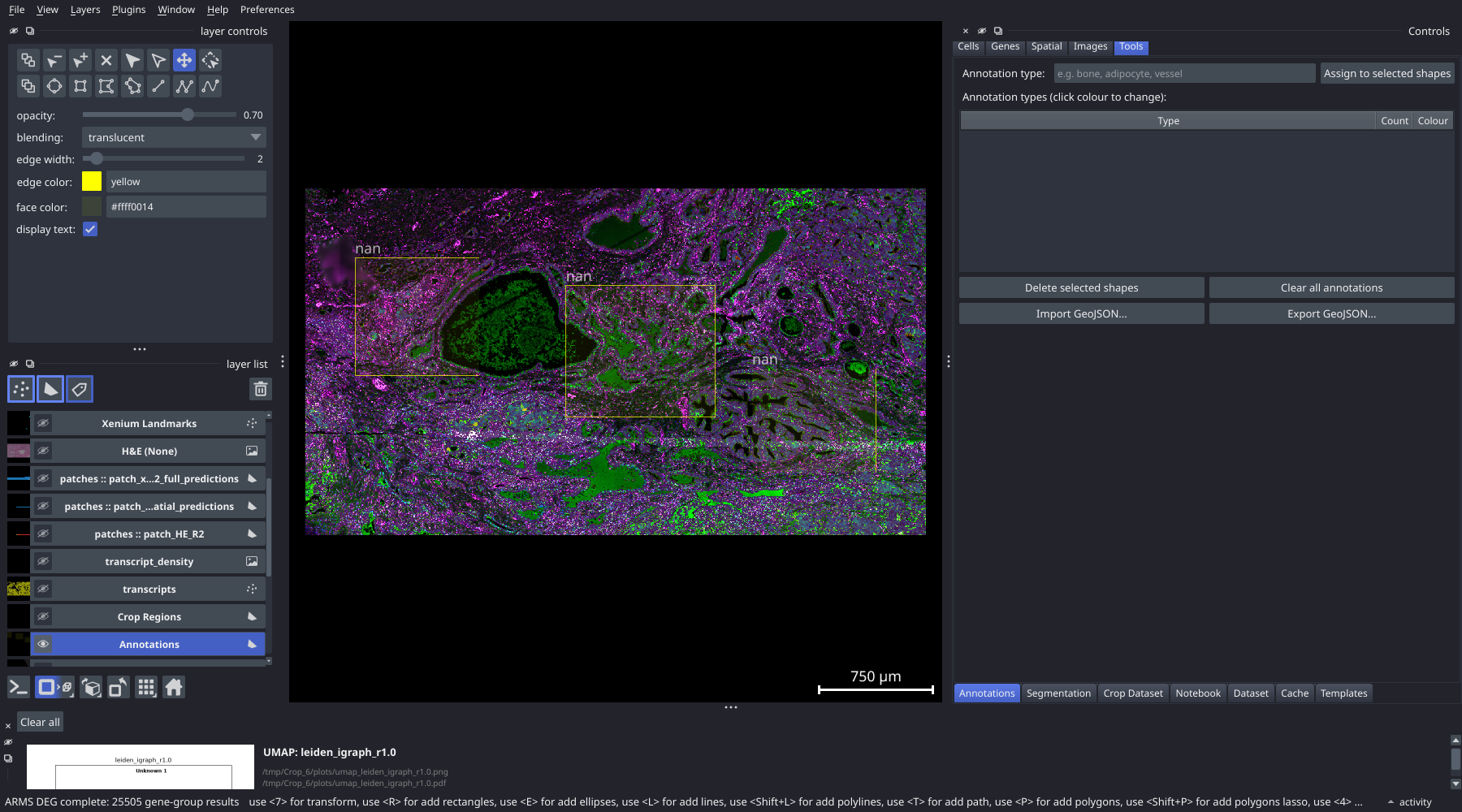
In the napari layer list on the left, click on the Annotations Shapes layer to make it active. The layer highlights to show it is selected.
Select the polygon tool in the napari toolbar (or press P). Click to place each vertex of your region boundary. Press Enter to close and finalise the polygon.
Repeat for each tissue region you want to annotate. You can draw multiple polygons before assigning types — the type assignment step is done separately.
Tips:
- Use the rectangle tool (
R) for quick rectangular regions. - Zoom in before drawing fine boundaries; zoom out for large tissue compartments.
- If you have a registered H&E image, use it as a visual guide while keeping the Annotations layer active.
In the control panel, go to Tools and click the Annotations tab.
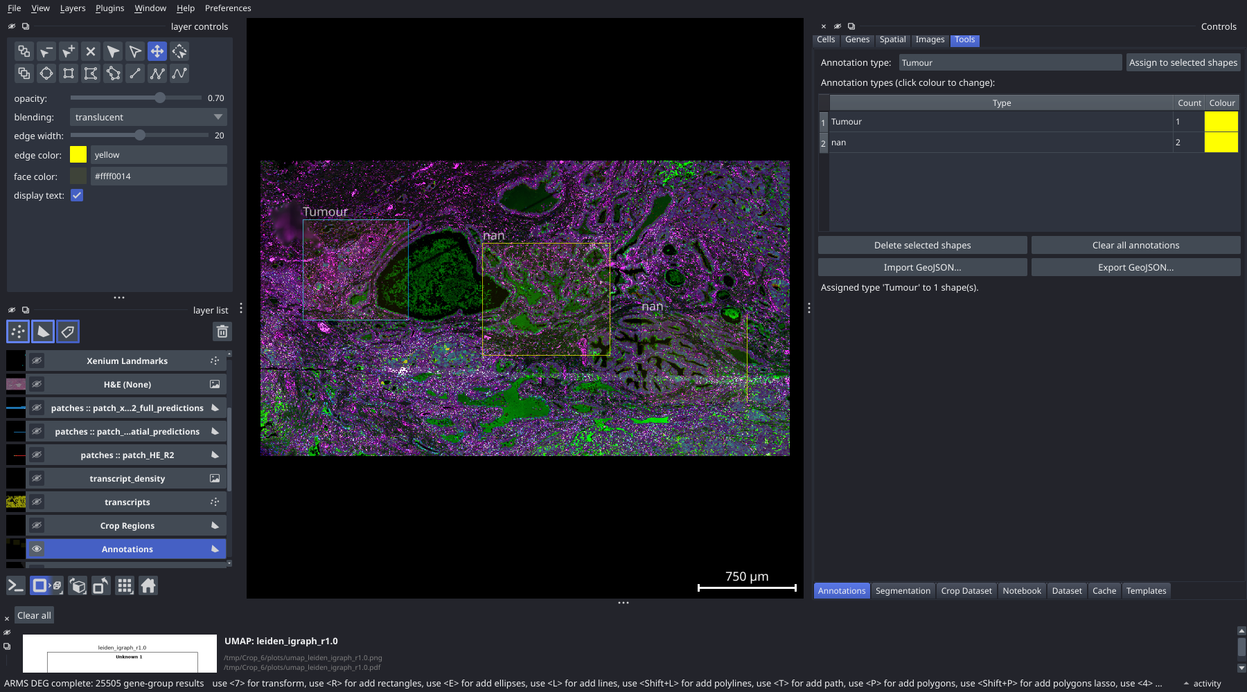
a. In the napari canvas, click a polygon to select it. Hold Shift and click to select multiple polygons of the same type.
b. In the Annotation type: text field in the Annotations tab, type a label (for example tumour, stroma, vessel, or necrosis).
c. Click Assign to selected shapes.
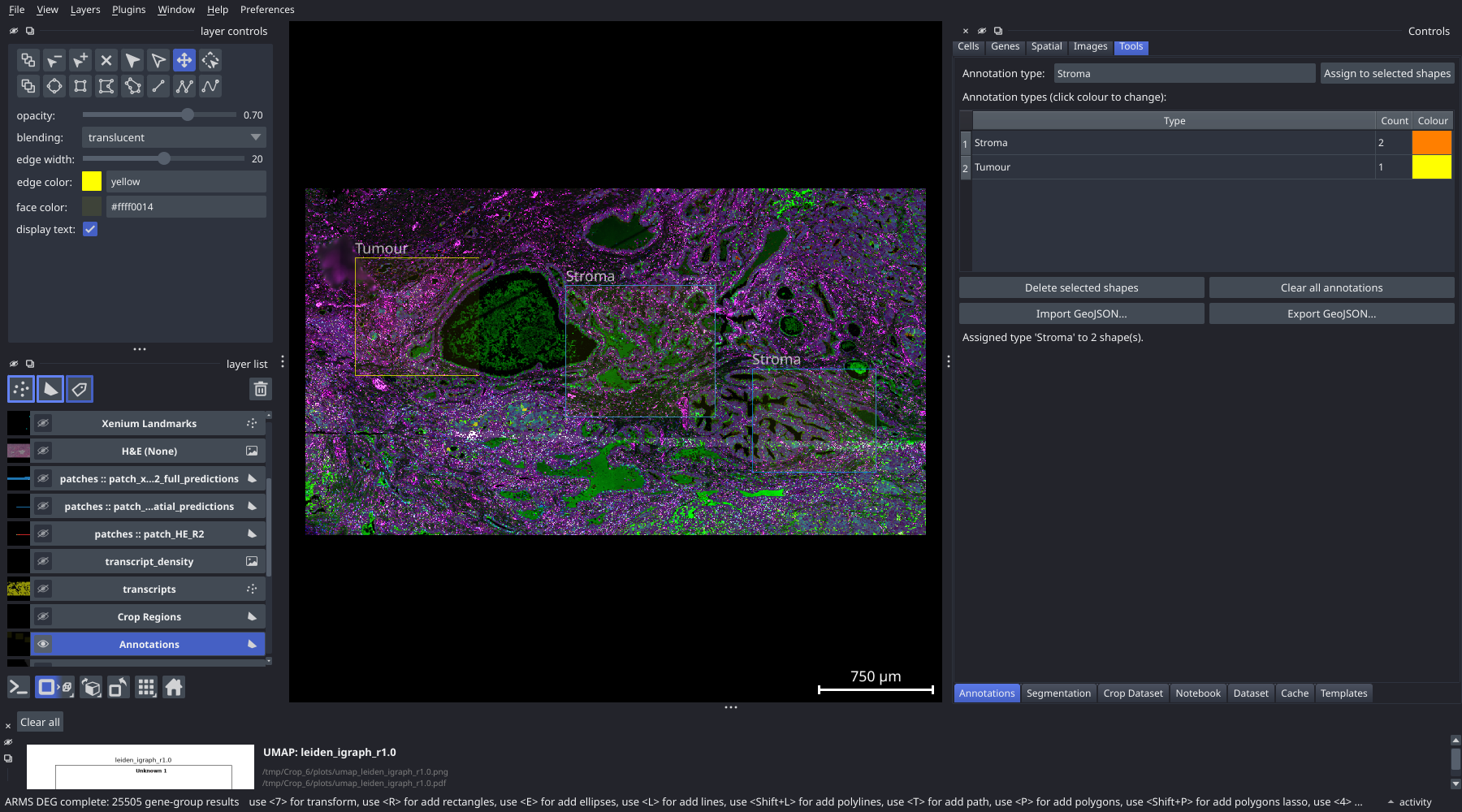
The type table below updates to show each defined type with a count of how many shapes carry that label.
In the type table, click the colour cell next to a type name to open a colour picker. Choose a colour that distinguishes the type clearly from the canvas background and from other annotation types. The polygon fill colour updates on the canvas immediately.
Repeat steps 2–5 for each tissue region type you need. Work through the tissue systematically — for example, annotate all tumour regions first, then all stroma regions.
Click Export GeoJSON... and choose a save path. The exported file contains:
- One GeoJSON Feature per polygon
- Each feature's
propertiesobject includes theannotation_typeand the assigned colour
The coordinates are in the Xenium pixel coordinate system. To convert to physical micrometres, multiply by the pixel size (typically 0.2125 µm/pixel, found in experiment.xenium).
To load annotations saved in a previous session or shared by a collaborator:
- Select the Annotations layer in the layer list.
- In the Annotations tab, click Import GeoJSON... and select the file.
Imported shapes are appended to any existing annotation polygons. Type assignments and colours are restored from the file.
| Action | How to do it |
|---|---|
| Remove selected shapes | Select shapes in the canvas, then click Delete selected shapes in the tab |
| Remove all annotations | Click Clear all annotations (a confirmation dialog appears before anything is deleted) |
| Rename a type | Re-select the shapes and assign a new type name; the old type disappears from the table if no shapes carry it |
| Change a shape's type | Select the shape(s) and click Assign to selected shapes with the new type name |
- Annotations are saved automatically to
sdata_cached.zarrwhen you close the viewer and restored on the next launch. - Annotation types defined here appear in the Annot Nhood and Annot Dist tabs, where you can measure cell-type enrichment and distance relationships relative to each annotation class.
- Overlapping polygons of different types are allowed; each polygon is treated independently in spatial analysis.
- GeoJSON files can be opened in QGIS, Python (
geopandas), or R (sf) for further processing.
- Tutorial-ROI-Analysis — draw ROI polygons for differential expression analysis
- Tab-Neighborhood-Enrichment — compute cell-type neighbourhood enrichment relative to annotation regions
- Interface-Overview — full reference for all control panel tabs