Tutorial Getting Started
Prerequisites: PALMS installed; a Xenium output directory available (containing experiment.xenium)
Time required: ~10 minutes
Run the viewer from the terminal, passing the path to your Xenium output directory:
palms /path/to/xenium/output/If you omit the path, a file dialog opens so you can select the directory interactively:
palms
On the first launch, the viewer builds a zarr cache (sdata_cached.zarr/) inside your output directory. This takes 3–10 minutes depending on dataset size, and on a full slide the cache is around 14 GB, so make sure there is room. Subsequent launches use the cache and take only 10–30 seconds.
A progress bar appears in the terminal and at the bottom of the viewer window while loading. The terminal also reports memory per element as each one is written — a full slide peaks around 9 GB and stays flat across the write.
If the dataset directory is read-only, or you only want a quick look, --no-cache will start without writing anything. On a full slide it is expensive rather than merely slower: see Memory in Installation before reaching for it.
Once loaded, use the following controls to move around:
| Action | Control |
|---|---|
| Pan | Middle-click drag, or Ctrl+drag |
| Zoom | Scroll wheel |
| Fit image to window | Press Space |
| Reset zoom | Press Ctrl+Shift+H |
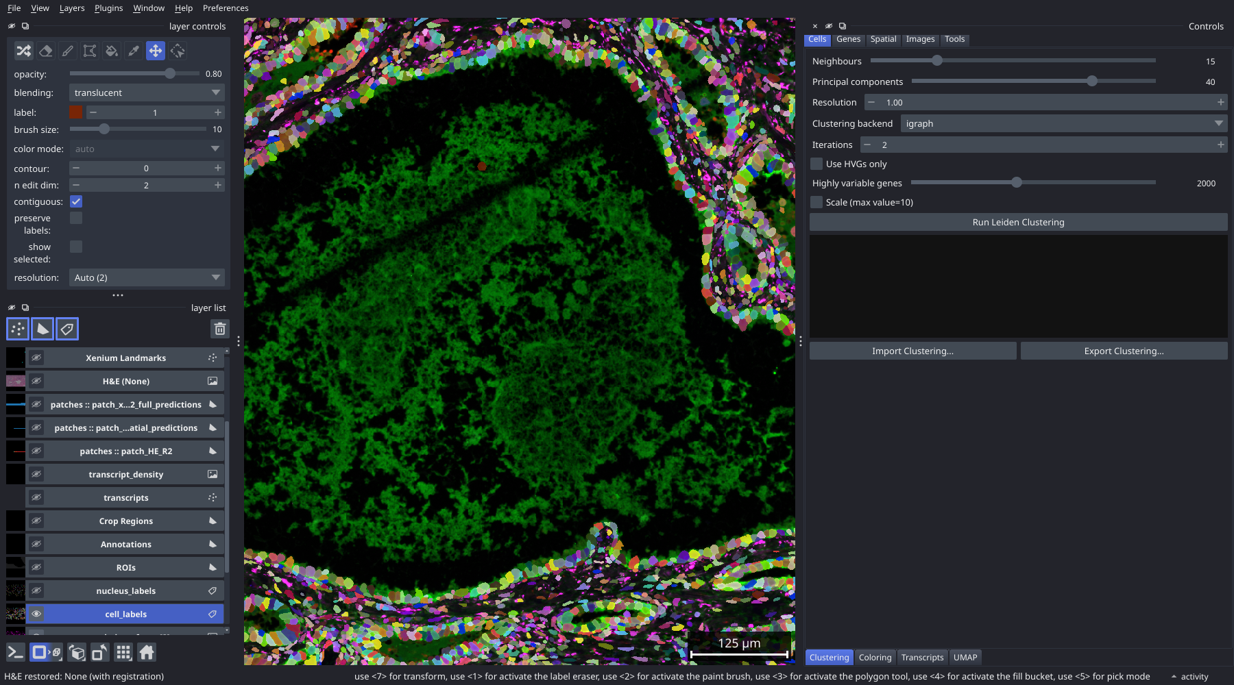
The default image layer (morphology_focus) is a 4-channel fluorescence image with the following channels:
| Channel index | Stain |
|---|---|
| 0 | DAPI |
| 1 | ATP1A1 / CD45 / E-Cadherin |
| 2 | 18S |
| 3 | AlphaSMA / Vimentin |
You can toggle individual channels on and off by clicking their eye icons in the layer list on the left side of the napari window. Adjust brightness and contrast with the sliders that appear when a layer is selected.
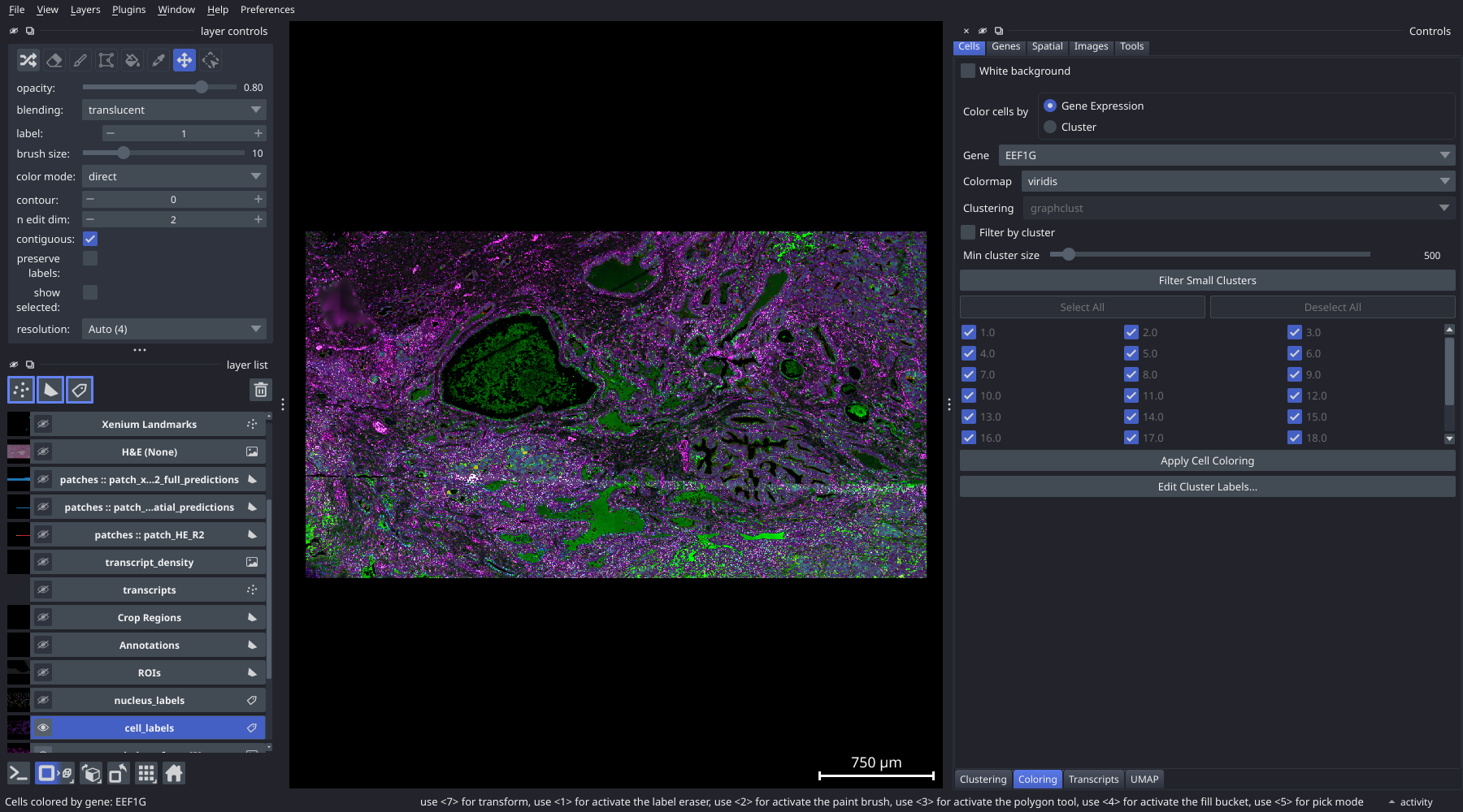
- In the control panel on the right, open the Cells group and click the Coloring tab.
- Set the Colour by dropdown to Gene Expression.
- Choose a gene from the gene dropdown.
- Select a colour map (e.g.
magmaorviridis). - Click Apply Cell Coloring.
The cell label layer updates to reflect per-cell expression levels.
- Open the Transcripts tab (Cells group).
- Select a gene from the Transcript gene dropdown.
- Click Add Gene to add it to the list.
- Click Apply Transcripts.
Individual transcript dots appear on the canvas. Use the Min QV slider to filter out low-quality transcripts (quality value below the threshold).

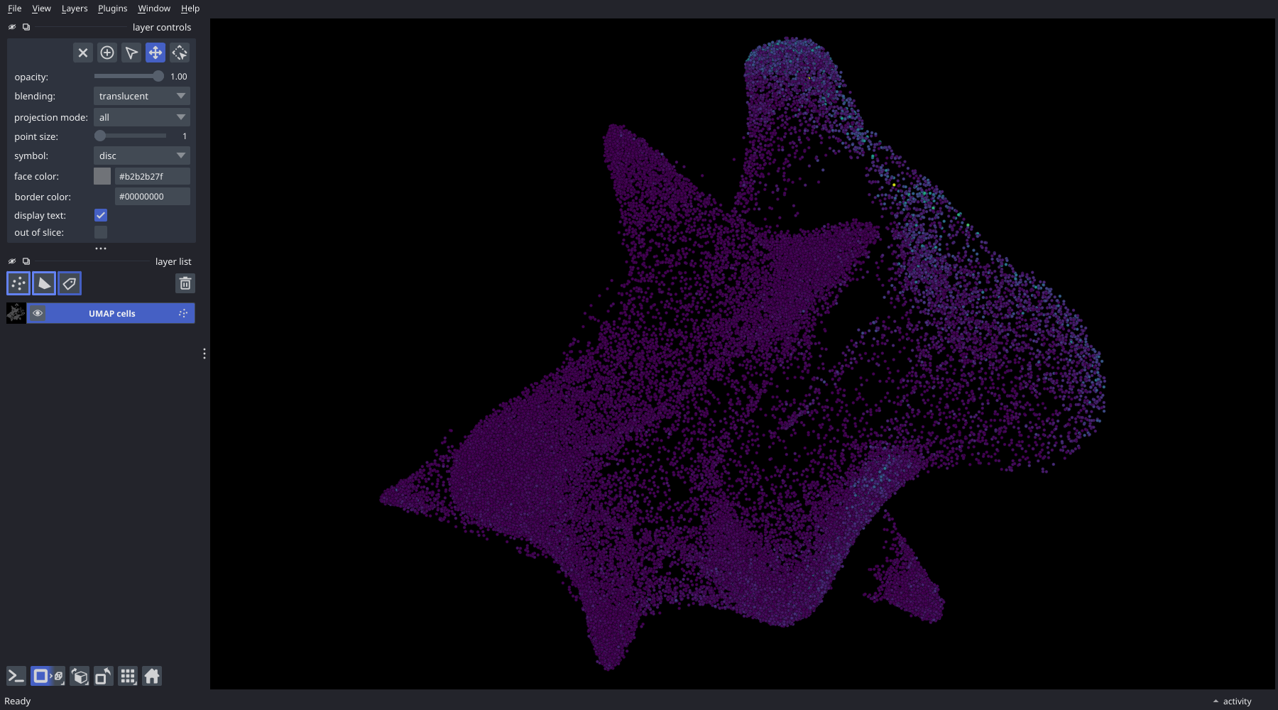
- Open the UMAP tab (Cells group).
- Click Show UMAP Window.
A separate window opens showing a scatter plot of the cells in UMAP space, linked to the main canvas. Lassoing cells in the UMAP highlights them on the spatial canvas, and vice versa.
Close the napari window normally (click the X or press Ctrl+Q). Your session — including the current clustering, gene selection, H&E registration, and ROI polygons — is saved automatically and restored the next time you launch the viewer on the same dataset.
- Tutorial-Clustering — run Leiden clustering and differential expression
- Tutorial-HE-Registration — register an H&E image to the Xenium canvas
- Interface-Overview — full reference for every control panel tab