Visualization

Visualization (CHESSPlots)

Folder: CHESS_Library/Visualization/ Entry point: CHESSPlots.m, a factory that returns the plotting object for the run's workflow.

The plotting classes draw CHESS inputs and results: the PSE profile, storm database contents, hazard curves, life-cycle damage and deterministic storm-by-storm results. The GUI Results, PSE and Storm DB tabs call these same methods, so a plot made from a script looks like the plot in the app.

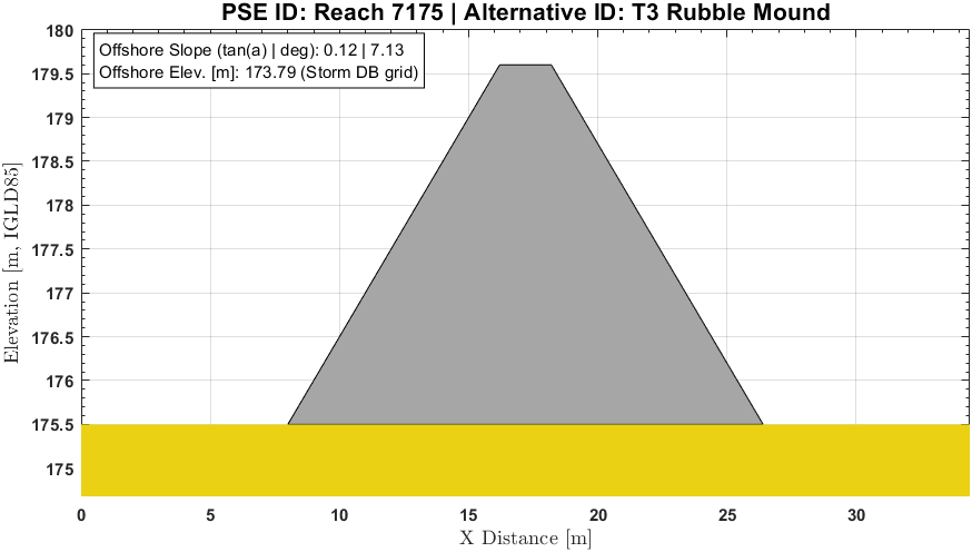
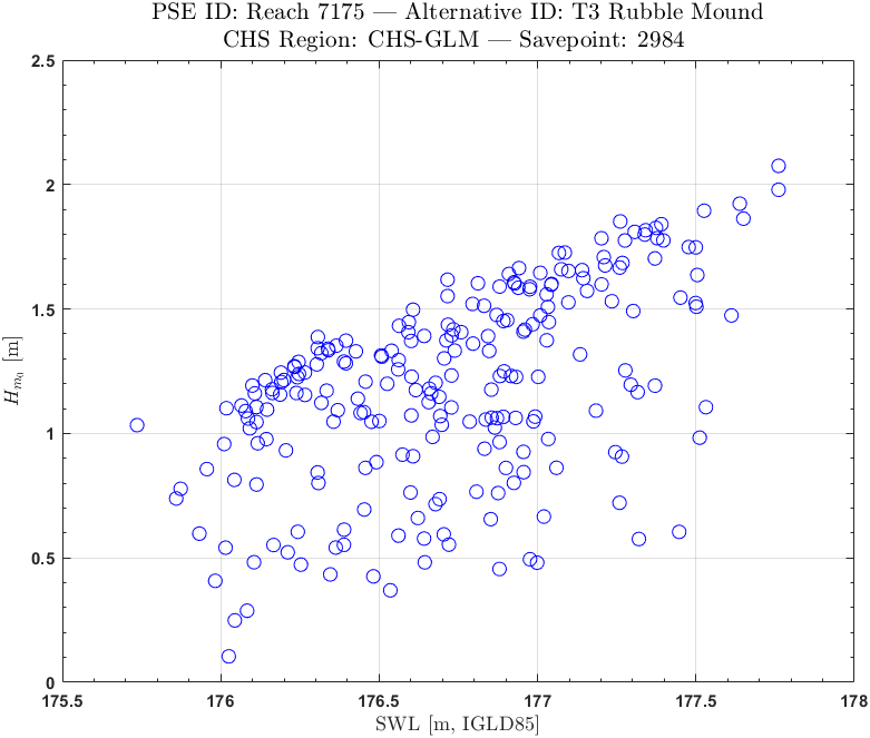
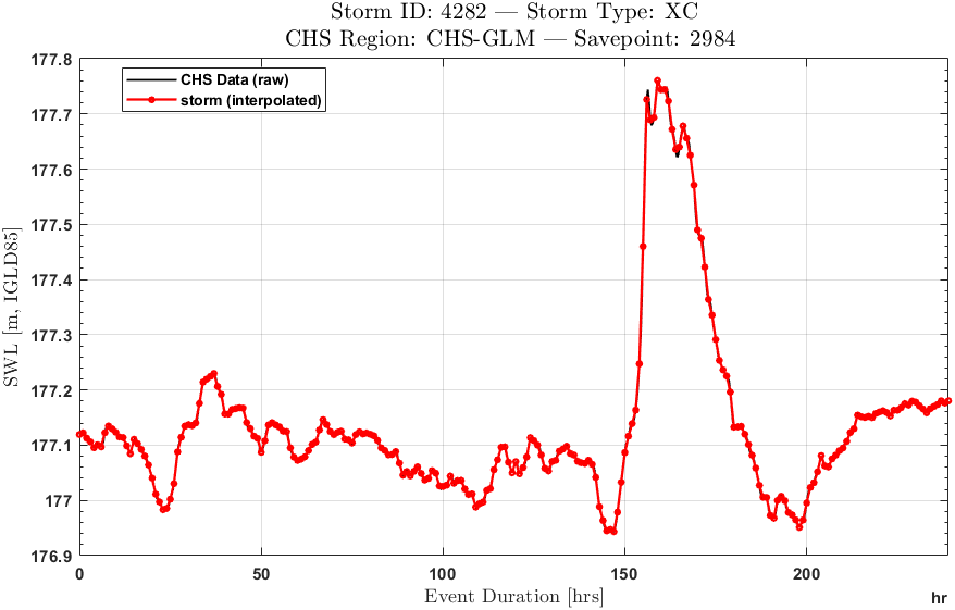
All example images on this page come from the code as it stands. They use the Chicago GRR storm database (CHS-GLM savepoint 2984, XC storms, IGLD85 datum) and an example rubble mound PSE (crest 179.6 m, toe 175.5 m, 1:2 slopes, 400 kg armor). PROS, LCS (300 life cycles × 50 years) and DET were each run on it.

Class layout

File	Class	Use
CHESSPlots.m	factory function	Returns the object for config.workflow
CHESSPlotsBase.m	CHESSPlotsBase	Shared properties and the input-screening plots (PSE, storms, single events). Every workflow class inherits these
pros_methods.m	pros_methods < CHESSPlotsBase	PROS hazard curves (workflow = 1 or 4)
lcs_methods.m	lcs_methods < CHESSPlotsBase	Life-cycle plots and dashboards (workflow = 3)
det_methods.m	det_methods < CHESSPlotsBase	Deterministic storm-by-storm plots (workflow = 2)
aux_methods.m	aux_methods (static only)	Data access, axes set-up, LaTeX escaping, unit symbols
chess_colormap.m	function	Colormap for the LCS annual distribution plots

CHESSPlots picks the class:

config.workflow	Returned object
1 (PROS), 4 (PROS-FB)	pros_methods
2 (DET)	det_methods
3 (LCS)	lcs_methods
anything else	error CHESSPlots:unsupportedWorkflow

Creating a plotting object

sp = CHESSPlots(config, Resp, storm, project_forcing, dsw, structure, base_fnt, unit_system);

Input	Content	Where it comes from
config	Run configuration	<db>_<workflow>_config_file.mat (config)
Resp	Project responses	<db>_<workflow>_project_responses.mat (Resp)
storm	Storm database storms	Storm DB .mat (storm)
project_forcing	Replicates (PROS), life cycles (LCS) or storms (DET)	<db>_<workflow>_project_forcing.mat
dsw	Storm probability masses (TC)	Storm DB .mat (prob_mass)
structure	PSE geometry and properties	<db>_<workflow>_config_file.mat (structure)
base_fnt	Base font size (titles are base_fnt + 2, ticks base_fnt − 2)	e.g. 12
unit_system	'SI' or 'Imperial' (axis unit symbols)

File locations are listed in Model Outputs. Pass [] for any input a plot does not use. For example, the Storm DB tab builds a CHESSPlotsBase with only config and storm.

Most methods also take a dataset query:

ds_query = struct('storm_type', 'XC', 'data_type', 'Peaks', 'match_type', 'Default');

Field	Values
storm_type	'XC', 'TC' or 'CC'
data_type	'Peaks' or 'Timeseries'
match_type	'Default', 'WLP' or 'WHP' (Timeseries always reads 'Default')

Where plots are drawn

The first input of a plot method is its target:

• Single-panel plots take an axes (axes, uiaxes), a figure or a grid layout. An empty or deleted target opens a new 1000 × 600 uifigure.
• Multi-panel plots (storm_event_viewer, mound_damage_dashboard, sampling_scheme_dashboard) take a figure, a grid layout or an axes. subplot_manager builds the panels: a tiledlayout in a classic figure, a uigridlayout in a uifigure.

f  = figure('Color', 'w');
ax = axes(f);
sp.hc_plot(ax, ds_query, 'R2p', 0);
exportgraphics(f, 'hc_r2p.png', 'Resolution', 150);

Titles and axis labels use the LaTeX interpreter. Labels, units and log scaling for each field come from response_library_headers.m.

---

Shared plots (CHESSPlotsBase)

Available from every workflow object.

pse_transect_plot

[ax, Geo] = sp.pse_transect_plot(ax, [])

Draws the PSE cross-section from structure: the bed (yellow), the structure (grey) and the toe berm when add_toe_berm = 1. Elevations are drawn signed, in the project datum. The box at the top left shows the offshore slope and the offshore elevation with its source (for example Storm DB grid), or n/a when none is set. Levees, rubble mounds and low-crested breakwaters use their seaside and leeside slopes; floodwalls are drawn as a vertical block. Geo is the structure polyshape. The third input is ignored and kept only so older calls still work.

storm_data_space_plot

ax = sp.storm_data_space_plot(ax, ds_query, var_left, var_right)

Scatter of storm peaks from the storm database: var_left (y axis) against var_right (x axis), one point per storm. Both are "SWL", "Hm0" or "Tp". Each storm's peak is the maximum of its record, so for Timeseries the two values can come from different hours. The title adds the PSE line only when config.struc_id is set.

event_hydrograph_plot

ax = sp.event_hydrograph_plot(ax, ds_query, event_id, field_to_plot, chs_data)

One storm's hydrograph from the storm database (red, interpolated to the CHESS time step). field_to_plot is "SWL", "Hm0" or "Tp". data_type is forced to Timeseries. When chs_data is given (the CHS_Data variable of the storm database _raw_files.mat), the raw CHS signal is drawn in black over the same window: ADCIRC for SWL, the wave model for Hm0 and Tp. For TC storms with tc_bias_corrected = 1, the raw SWL is bias-corrected the same way as in call_chs_storm_quality_check, and the legend says so. The x axis is elapsed hours.

storm_event_viewer

sp.storm_event_viewer(parent, ds_query, event_id, response_to_view, datum_offset)

Two-panel view of one storm (Timeseries) or of every storm (Peaks, event_id ignored), with a structure response recomputed for it:

• Top: SWL, PSE crest, Hm0 before (dashed) and after (solid) depth limitation, toe depth h, freeboard Rc, and the berm depth when there is a toe berm. Click a legend entry to hide or show its line.
• Bottom: the requested response.

The response is recomputed, not read from Resp. The method rebuilds PROS forcing from storm without replicates (chess_pros_formater), applies adjust_project_forcing with depth limitation forced on, switches on every compute_* flag and calls compute_structure_response. Sea level change and tides follow config; for LCS runs, a fresh tide draw is used because LCS tide indices belong to life cycles, not storms. The responses allowed depend on structure.struc_type; an unsupported one raises an error that lists the allowed set.

datum_offset is subtracted from SWL and the crest only. Use it when the datum puts water levels far from zero (Great Lakes IGLD85 here), or SWL and the crest flatten the other lines. The y-axis label keeps the project datum name. Pass 0 (or []) for no offset.

With data_type = 'Peaks', the x axis is the storm number and the response is drawn as one marker per storm:

subplot_manager

[gl, subplot_flag] = sp.subplot_manager(parent, nRows, nCols)

Helper used by the multi-panel plots. With a classic figure or an axes it builds a tiledlayout and returns an array of axes (subplot_flag = true). With a uifigure, a grid layout or a uiaxes it returns a uigridlayout (subplot_flag = false), and the caller places each axes by row and column.

---

PROS plots (pros_methods)

PROS Resp holds, per dataset and storm type, a struct array with one element per hazard curve (var = field name, x_plot/y_plot for drawing, x_table/y_table for tables, CL, title, y_label, y_log_scale). The forcing curves are SSL (SWL), Hm0 and Tp when pros_compute_forcing_HC = 1 (CHESS PROS).

hc_plot

ax = sp.hc_plot(ax, ds_query, field_to_plot, add_events)

The hazard curve of field_to_plot: best estimate (solid black) and up to four confidence levels from project_CLs (dashed). The x axis is AEF (10^0 to 10^-4) or AEP (10^0 to 10^-3) as set by pros_use_aep, drawn in reverse. The y axis is log when the field's y_log_scale = 1 (e.g. q). A field that is not in Resp gives an empty axes with the "No data available" note.

add_events = 1 overlays each storm of the record as a green marker on the best-estimate curve. Each storm's response is recomputed from project_forcing without replicates (*_no_rep) and compute_structure_response; for SSL/SWL, Hm0 and Tp the forcing value itself is used. The AEF of each marker comes from get_aef (below). This needs project_forcing, and TC also needs dsw (TC_Freq).

frequency_base_comparison_plot

[ax, fb_data] = sp.frequency_base_comparison_plot(ax, ds_query, field_to_plot)

Draws the response-based (RB) hazard curve with hc_plot, then runs PROS-FB on the same run and adds the FB curves as dotted lines. PROS-FB (chess_pros_frequency_base) computes the response from the SSL, Hm0 and Tp hazard curves taken at the same frequency, so the run needs pros_compute_forcing_HC = 1. The plot writes no files; FB output names point to <workflow folder>/FB1 (Peaks) or FB3 (Timeseries). fb_data returns the FB curves of the storm type.

FB assumes the water level and wave height of a given frequency happen together, so it is usually above RB, as here. The y limits are widened to fit both the RB and FB curves. If PROS-FB has no curve for the requested field, the RB curves are kept and no FB lines are added.

get_aef

[data_out, idx] = sp.get_aef(response_vector, benchmark_aef, benchmark_hc, dsw, resp_indx)

Gives each storm response an AEF. Used by the event overlay.

• XC (dsw empty): log(AEF) is interpolated on the hazard curve (benchmark_hc against benchmark_aef). Responses outside the curve take the end values. Non-finite and repeated curve points are dropped first.
• TC (dsw = one probability mass per storm, same size as response_vector): storms are sorted by response, largest first, and AEF is the running sum of their masses.

data_out has aef, response (sorted, largest first) and resp_indx; idx is the sort order.

---

LCS plots (lcs_methods)

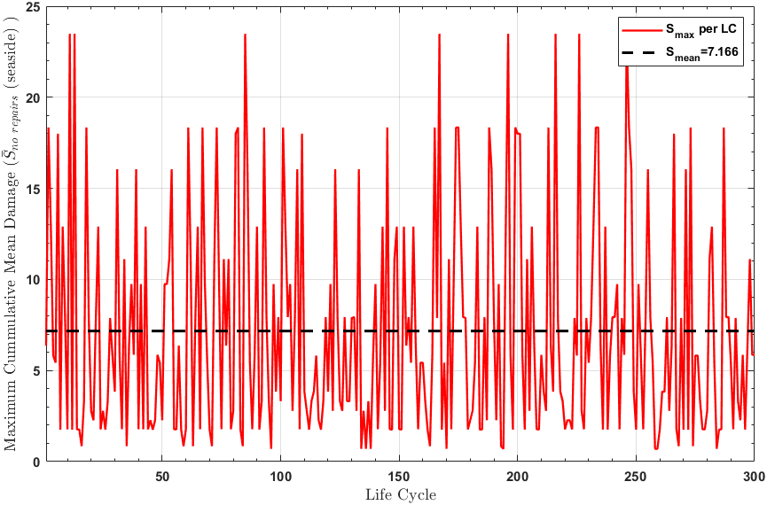
LCS project_forcing holds one array per life cycle; LCS Resp holds one response series per life cycle, plus S (damage progression, rubble mounds only) for Timeseries runs (CHESS LCS). The armor damage plots need structure.struc_type = 3 and a Timeseries run with seaside or leeside Dn50 switched on.

The example run is XC only, 300 life cycles of 50 years, full Poisson sampling.

slope_armor_damage_plot

ax = sp.slope_armor_damage_plot(ax, ds_query, field_to_plot, lc_index)

Cumulative armor damage S from Resp.Timeseries.Default.<storm_type>.S. data_type is forced to Timeseries.

field_to_plot	Draws
S_seaside_no_repairs, S_seaside_with_repairs, S_leeside_no_repairs, S_leeside_with_repairs	One line per life cycle against the time step of the life cycle. lc_index picks life cycles ([] = all)
Smax, LSmax	Mean damage across life cycles against simulation year (dashed black). lc_index does not apply

This method only draws lines. It does not set up the axes (no title, labels or hold on), so call hold(ax, 'on') first, as the GUI Results tab does, or each life cycle replaces the one before. A PSE that is not a rubble mound raises an error.

plot_mound_final_damage_state

ax = sp.plot_mound_final_damage_state(ax, ds_query, field_to_plot)

Final damage of each life cycle (red) and its mean (dashed black, value in the legend). field_to_plot is S_seaside_no_repairs or S_leeside_no_repairs; without repairs, damage only grows, so the last value is the maximum. Life cycles with no storms keep S = 0. Timeseries only.

plot_mound_damaging_instances_distribution

ax = sp.plot_mound_damaging_instances_distribution(ax, ds_query, field_to_plot)

For each life cycle, the share of time steps in which damage grew, split by structure state: emergent (blue bars) or submerged (red line, SWL above the crest). field_to_plot is any of the four S_* series. For the *_with_repairs series, damaging steps are found storm by storm, comparing with the damage at the end of the previous storm.

plot_pse_submergance_distribution

ax = sp.plot_pse_submergance_distribution(ax, ds_query, use_log_x, is_count, cb_log, cb_lim)

How long the structure is submerged (SWL above the crest) per storm, binned by simulation year. Hours under water per storm are counted, then binned with compute_annual_distribution and drawn with plot_annual_distribution (see below). use_log_x sets a log x axis, is_count shows counts instead of percentages, cb_log and cb_lim set the colour scale.

In the example, the SWL never reaches the crest, so every storm falls in the 0-hour bin:

annual_response_distribution

[ax, bin_data] = sp.annual_response_distribution(ax, ds_query, field_to_plot, bin_edges, norm_type, cb_lim, grid_on, cb_log)

Distribution of storm peak responses by simulation year. For each storm in every life cycle, the maximum response is taken and assigned to the year the storm falls in (compute_lcs_yearly_curve). Each year's values are binned:

Input	Use
field_to_plot	Any response computed by the run (R2p, q, Dn50, p1, ...) or an S_* damage series
bin_edges	Inner bin edges. [] makes 5 edges between the minimum and maximum (generate_bin_guess; log spacing for log-scale fields)
norm_type	"percent" (share of the year's storms) or "count"
cb_lim	Colour limits ([] = data range)
grid_on	Kept in the signature; not used by the method
cb_log	Log colour scale

Two extra bins catch values below the first edge and above the last (x <= ..., x >= ...). Empty bins are blank. bin_data returns the plotted values (one row per year). A field that is all NaN gives an axes with "No finite response values to plot".

The building blocks are public:

Method	Use
generate_bin_guess(resp_vector, n_bins, use_log)	Evenly spaced (or log-spaced) edges from the global minimum to maximum. A constant response is padded so there are always two edges
compute_annual_distribution(stm_data, resp_vector, nYears, x_scale_log, is_count, bin_edges)	Bins the yearly values and returns bin_data and the plotted edges
plot_annual_distribution(ax, bin_data, bin_edges, use_log_x, is_count, cb_log, cb_lim)	Draws the pcolor grid with the chess_colormap colours and the colourbar

event_sampling_distribution

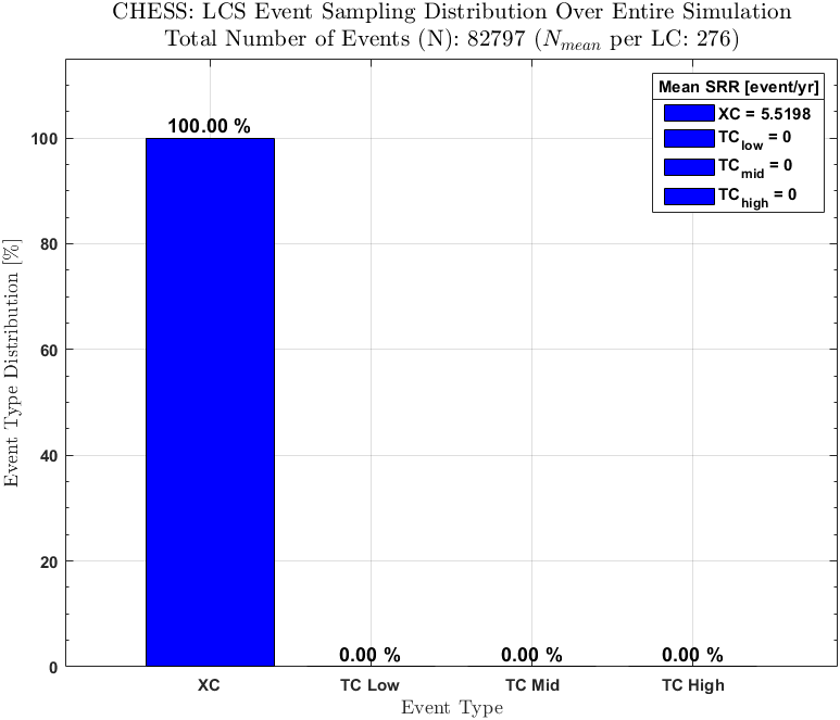
ax = sp.event_sampling_distribution(ax, ds_query, lc_index)

Share of sampled storms by type (XC, TC low, TC mid, TC high) over all life cycles, or over the life cycles in lc_index. The legend gives each type's mean storm recurrence rate (storms per year), and the title gives the total number of storms and the mean per life cycle.

mound_damage_dashboard

sp.mound_damage_dashboard(parent, ds_query, field_to_plot, s_bin_edges, s_cb_lim)

Five panels for one damage series (S_seaside_* or S_leeside_*):

Panel	Plot
Top left	plot_mound_damaging_instances_distribution
Top right	plot_pse_submergance_distribution (percent, linear)
Bottom left	slope_armor_damage_plot with Smax (seaside) or LSmax (leeside)
Bottom middle	plot_mound_final_damage_state (no-repairs series of the same side)
Bottom right	annual_response_distribution of field_to_plot with s_bin_edges and s_cb_lim

sampling_scheme_dashboard

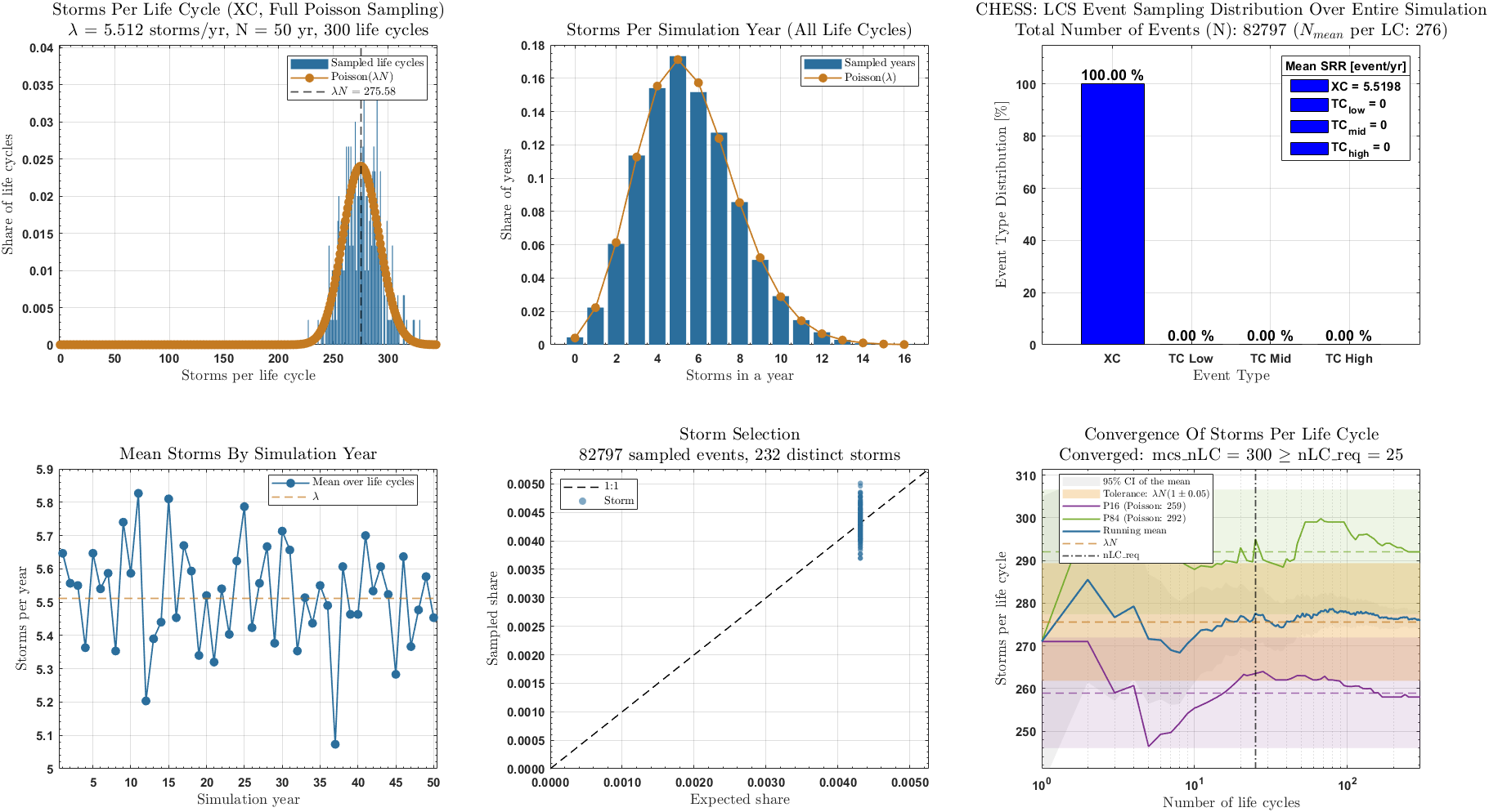
sp.sampling_scheme_dashboard(parent, ds_query)

Six panels that check the LCS storm sampling for one storm type:

1. Storms per life cycle against Poisson(λN). With rate-matched sampling (lcs_restrict_sampling_rate = 1), the λN ± 1 window is shaded.
2. Storms per simulation year, all life cycles together, against Poisson(λ).
3. Event type mix (event_sampling_distribution).
4. Mean storms by simulation year, against λ. Shows whether storms are spread evenly through the life cycle.
5. Storm selection: share of samples for each storm against the expected share. XC storms are drawn evenly, so the expected share is 1/Nstm_XC. For TC it is the intensity bin rate times the storm's frequency within the bin, which needs dsw and storm.
6. Convergence over the number of life cycles: running mean and running percentiles (project_CLs) of storms per life cycle. With full Poisson sampling, this also shows the targets of lcs_convergence_check (λN within the tolerance, Poisson percentiles), the required number of life cycles nLC_req and the verdict. The stored result config.lcs_convergence_results is used when present. Rate-matched sampling has no targets and no check.

λ is Nstm_XC/Nyrs_XC for XC, and dsw.TC_SRR(end) for TC (or the sample mean when dsw is missing). The sampling mode comes from lcs_sampling_mode(config).

Other public helpers

Method	Use
split_into_events(ds_query, value_in)	Splits each life cycle's series into one cell per storm (Timeseries: storms start where column 10 is 0)
get_damaging_instances(ds_query, field_to_plot)	Damage values and time-step indices where an S_* series grows

---

DET plots (det_methods)

DET Resp holds the full history of every field for each storm plus a Max table with one value per storm (CHESS DET). Any forcing field (SWL, Hm0, Hm0_DL, Tp, h, Rc) or computed response can go on any axis.

available_fields

fields = sp.available_fields(ds_query)

Names that can be plotted for the dataset: forcing first, then responses. For the example run: SWL, Hm0, Hm0_DL, Tp, h, Rc, R2p, R2p_SWL, q, q_wave_ot, Dn50, Dn50_Lee, Hm0t.

response_vs_forcing_plot

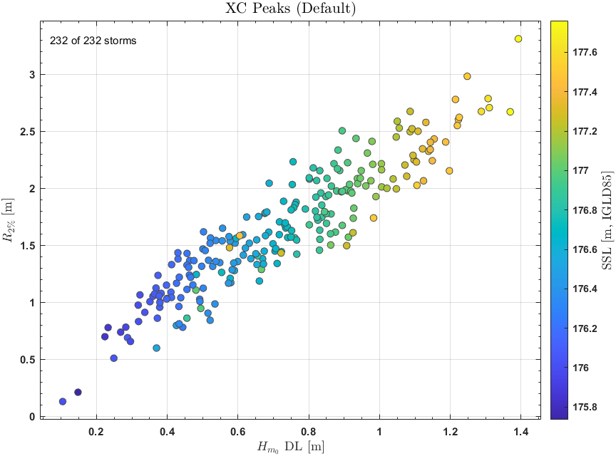
ax = sp.response_vs_forcing_plot(ax, ds_query, x_field, y_field, c_field)

One point per storm: x_field against y_field, coloured by c_field. Peaks use each storm's single value. Timeseries use the storm maxima, taken field by field, so the x and y values can come from different hours; Rc uses its minimum. Storms with a NaN in any of the three fields are dropped, and the count kept is shown at the top left. Log scales follow response_library_headers. An unknown field raises det_methods:unknownField with the list of available fields.

peaks_vs_timeseries_plot

ax = sp.peaks_vs_timeseries_plot(ax, ds_query, field)

The same field from the Peaks run (x) and the Timeseries run (y), matched by storm ID, with a dashed 1:1 line. Peaks use ds_query.match_type. The run needs both datasets (use_peaks = 1 and use_timeseries = 1), otherwise det_methods:missingDataset is raised. Points below the line mean the time-varying storm gives a smaller peak than the single Peaks record, for example because the SWL and Hm0 peaks do not happen at the same hour.

response_table

fig = sp.response_table(ds_query, storm_id)

Opens a uifigure with a plot above a table.

• Peaks: one row per storm. Select two columns: the first click sets the x axis, the second the y axis.
• Timeseries: pick a storm in the Storm ID list (or pass storm_id). The table shows its hourly rows, and the selected columns are drawn as hydrographs. Datum elevations (SWL, R2p_SWL, DamDepthElev) and other fields are grouped by unit; at most two groups can be shown (left and right y axes).

The table shows values rounded to 4 decimals, so small overtopping rates show as 0 in the table while the plot uses the full values. For scripts and tests, fig.UserData holds select(names), set_storm(id), axes and table:

f = sp.response_table(ds_query);
f.UserData.select({'Hm0_DL', 'q'});

---

Helpers (aux_methods)

Static methods, called as aux_methods.<name>(...).

Method	Use
pull_data(ds_query, ds)	Returns one dataset from storm (storm.(storm_type).(data_type).(match_type)) or from Resp / project_forcing (.(data_type).(match_type).(storm_type)). Timeseries always reads Default
initiate_axes(parent, x_label, y_label, title, base_fnt, row, col)	Creates or clears the axes and applies the CHESS style: grid, minor ticks, bold fonts, box, LaTeX title and labels, Tag = 'chess_fig'. row/col place it in a grid layout
latex_escape(str)	Escapes # % & _ $ ^ \ outside $...$ math so text is valid LaTeX. Already escaped text is unchanged
display_no_data(ax, base_fnt, msg)	Red "No data available" box (or msg) in the centre of the axes
pad_limits(ax, 'X'/'Y', data, frac)	Sets the axis limits to the data range plus a margin (5 % per side by default; decades on log axes)
tern(cond, a, b)	Returns a if cond, else b
build_unit_library(unit_system)	Unit symbols and conversion factors for 'SI' or 'Imperial'

Related pages

• Model Outputs: the files these plots read.
• CHESS PROS, CHESS LCS, CHESS DET: the workflows behind each plot class.
• GUI Quick Start: the same plots in the Results, PSE and Storm DB tabs.