Quest module configuration

The Quest module is basically a siguanet_quest client that provides access to the PostgreSQL functions in this SIGUANET extension. While functions in PostgreSQL do not define type behaviour, the classes behind Quest provide spatial types which invoke this functions in order to retrieve scalar and record data at different aggregation levels. You can think of it as a hierarchical object model giving you a multidimensional view of data in line with OLAP systems.

Understanding Quest object model

The spatial hierarchy in Quest object model is already implied in SIGUANET's database model and can be easily explained by decomposition of an enclosure identifier. Enclosures are the basic spatial entities and units of information in SIGUANET. Enclosures have a polygon geometry, belong to an organizational unit, may host people who work in them and are always assigned a primary purpose or use. They can be typically referred to as "rooms", although many of the enclosures in your SIGUANET database won't fall in this category (think about walls, elevators, staircases, outdoor facilities, ...). We may group enclosures attending to a spatial hierarchy and get aggregated information which describes higher level spatial entities. Speaking OLAP terminology, you can assume that Quest uses "geography" as the mandatory dimension for quantifying enclosures, people at workplaces, areas or rates.
By convention, enclosure identifiers are 9 characters long strings structured as a spatial thesaurus. Let's take the following enclosure identifier:

0037P1015

You should read it as:

00-37-P1-015

where:

{CAMPUS:'00', BUILDING:'37', FLOOR_LEVEL:'P1', ENCLOSURE:'015'}

and the FLOOR_LEVEL component value domain is:

(PB | P[1-9] | S[1-9])

where:

• PB stands for ground level
• P prefix stands for aboveground level
• S prefix stands for underground level

With this thesaurus in mind, we can directly infer 6 levels of spatial aggregation using simple SQL queries:

• the organization as a whole
• one floor level within the organization
• a particular campus
• one floor level within a particular campus
• a particular building
• a building floor

In short, Quest object model is built upon one interface and 6 implementing classes matching each one of the 6 aggregation levels. This interface provides a bunch of methods which are implemented by each class by invoking the suitable siguanet_quest functions. And that's all to it, basically! You just configure the Quest module by defining which methods of the interface are to be invoked for a particular user profile. This means you should be familiar with these methods, their parameters and their expected output. Once configured, the siguanet_quest client uses reflection to generate each aggregation level, that is to build instances for each of the classes implementing the interface and create the tree view for you at runtime. Detailed documentation on spatial aggregation methods is available at the Appendix A: The IUnidadGeoEstadistica interface.

Quest configuration editor

Remember that Quest module configuration is embedded in your profile definition documents. We'll assume you already are a Root user and got a Root profile stored in your minserve\ folder. If not, then go back to the Configuring user profiles page.
In this section we'll give a few configuration examples so that you can build upon them. Anyway, you should eventually consider having a look and using the .sgd files in the profile_samples\ folder. Let's begin by running siguanet-desktop with Minserve enabled:

> SIGUANETDesktop.exe --minserve

We'll be configuring Quest for your own profile, so access the application as Root. Next step is to expand the application modules tree and right click on the node corresponding to the Quest module configuration. You'll be presented with a context menu where each item allows creating a "data access point", as in the image below.

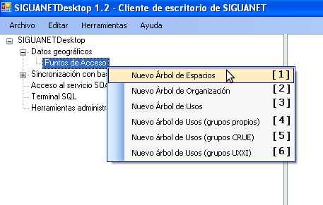
Within the Quest module, you should consider a data access point as a set of measurements (queries returning scalars) using one or two dimensions for aggregation purposes, being "geography" (spatial aggregation) a mandatory dimension in all cases. As of version 1.2, these are the available data access points (list numbers match the ones in the image above):

• [1] Raw Spatial Tree: aggregates data according to Quest's spatial hierarchy.
• [2] Organizational Tree: aggregates data according to organizational units; for each organizational unit, aggregates data spatially.
• [3] Functional Tree: aggregates data according to enclosure use or function; for each use, aggregates data spatially.
• [4] Functional Tree (SIGUANET classes): aggregates data according to enclosure use or function classes as defined by SIGUANET; for each class, aggregates data spatially.
• [5] Functional Tree (Universitas XXI classes): aggregates data according to enclosure use or function classes as defined by Universitas XXI ERP system; for each class, aggregates data spatially.
• [6] Functional Tree (CRUE classes): aggregates data according to enclosure use or function classes as defined by CRUE (Commitee of Chancellors of Spanish Universities); for each class, aggregates data spatially.

The Quest object model supports just one instance for each data access point, so you can have as many as 6 access points or different trees in one profile (this will normally be the case for Manager and Root profiles). Once a data access point is created you can configure its set of measurements as you wish, or even leave it empty. Should you need to recreate it, then delete it first and start from scratch. All access points or trees follow the same configuration guidelines. As an example, let's add and configure a few significant measurements for the Raw Spatial Tree now. Select the Raw Spatial Tree item in the context menu. A new node will be created under the Quest module configuration node. Next, have a look at the image below and follow the steps:

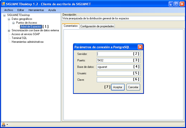
• [1] Select the newly created node. The Raw Spatial Tree is a data access point so whenever you select it the application will look for a PostgreSQL connection string. When you log in as a non Root user, the application stores the database connection parameters in memory after decrypting the corresponding .srs file. However, when you log in as a Root user there's no .srs and you are presented with a PostgreSQL connection dialog, as the one shown in the image.
• [2] In the PostgreSQL connection dialog, type your database server address.
• [3] Enter your PostgreSQL service port. Default port is 5432.
• [4] Supply your SIGUANET database name. Default name is siguanet.
• [5] Enter your PostgreSQL user name.
• [6] Type your PostgreSQL user account password.
• [7] Press the Accept button to resume.

If your connection parameters are correct you'll be able to test the measurements in your Raw Spatial Tree on the go. In case of connection failure, remember you can always modify PostgreSQL connection parameters by invoking the dialogue through the Editar > Conexión SIGUANET (PostgreSQL) item in the main menu.
Let's define your first measurement now. Suppose you want your Raw Spatial Tree to always get you informed about the number of teaching rooms and show them on a map. Here's how to do it:

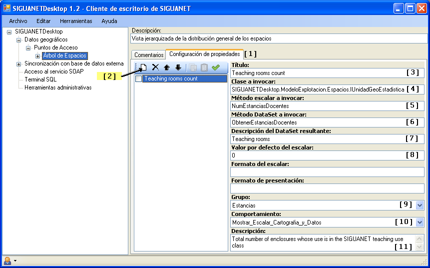
• [1] Select the measurement definition tab page.
• [2] Press the New Measurement button.
• [3] Enter the title that yo want to be displayed for this measurement, let's say Teaching rooms count.
• [4] Type the fully qualified name of the interface or class that holds the method that will be invoked. In practice, the Quest object model provides a single interface to hold every method giving you information about enclosures and employee locations that can be spatially aggregated. This interface is named IUnidadGeoEstadistica and its fully qualified name is supplied by default. Each class implementing it matches one of the 6 spatial aggregation levels. So, by using this interface what you're effectively instructing the application is to invoke the method on every instance of a class that implements this interface. If we focus on the GUI, what the user gets is a treeview with nodes representing different spatial aggregation levels. Whenever the user selects one of these nodes, the method gets invoked and the measurement output is displayed.
• [5] Enter the name of the scalar method that matches the measurement you need. In our case, this is NumEstanciasDocentes. The Appendix A: The IUnidadGeoEstadistica interface page lists all scalar methods available.
• [6] Enter the name of the collection method corresponding to your scalar method, which is ObtenerEstanciasDocentes in our example. In the Appendix A: The IUnidadGeoEstadistica interface page, you'll find the mapping between scalar and collection methods. Supplying the collection method is mandatory if you want a detail view of the enclosures or employee locations you're measuring. As you'll see in step [10], a detail view can be just tabular or include both, maps and data.
• [7] Since you provided a collection method, you should enter a string that briefly describes the objects in the result set. This description will be forwarded to the detail view window and will help to distinguish among several window instances. In our case, "Teaching rooms" will do the job.
• [8] Supply a default value just in case the measurement may fail. We'll use 0 here. If you don't want to mask error conditions, use a negative value instead.
• [9] Choose one category among General, Enclosures ( Estancias ) or Staff ( Personal ) so that related measurements are grouped in the GUI. Selecting the Enclosures category makes sense here.
• [10] Each measurement has an application behaviour in terms of usability. Possible behaviours are:
• Deshabilitado: this measurement is disabled so it won't show in the GUI.
• Mostrar_Escalar: the output of this measurement will be displayed as one line in the GUI.
• Mostrar_Escalar_y_Datos: clicking on this output's line a simple grid view will be displayed.
• Mostrar_Escalar_Cartografia_y_Datos: clicking on the this output's line a TreeMAP view will be displayed. This is a view that includes a tree view for navigating the result set retrieved by the collection method, together with an interactive map view, predefined legends, print preview and grid view.
• Mostrar_Escalar_y_Cartografia: clicking on this output's line a TreeMAP view will be displayed, but the grid view will be empty and users won't be able to browse tabular data.
  If you're measuring an absolute figure, as in our case, you will typically select Mostrar_Escalar_Cartografia_y_Datos, although we'll see an exception to this rule later on.
• [11] Type a comment on this measurement itself. It will render as a floating text when hovering over its line in the GUI so that you can help users to understand its meaning precisely.

What about measuring the area covered by teaching rooms? This is how you would do it:

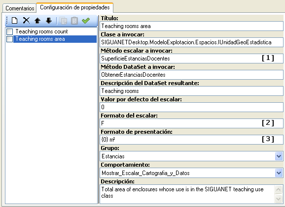
Remarkable points from the above screen capture are:

• [1] The suitable scalar method is SuperficieEstanciasDocentes. You'll find a whole bunch of area calculation methods in the Appendix A: The IUnidadGeoEstadistica interface page. Please note the collection method is the same that the one in the previous measurement and it makes sense: we are either counting enclosures or calculating areas, but both measurements refer to the same set of enclosures (teaching rooms).
• [2] You can specify a .NET standard numeric format for this measurement. In our case we used fixed point:

"F"

• [3] To make your measurement more readable, you can use a .NET composite format string and assume format item {0} refers to your measurement's value. Since we're using the square metre as our unit of measure, the format string is:

"{0} m²"

Let's move on from enclosures to people locations. Assume you want to know how many teachers and researchers are within your organization, their spatial distribution and eventually the floor plan directories showing offices or labs they work in. Here's how to configure a measurement for that:

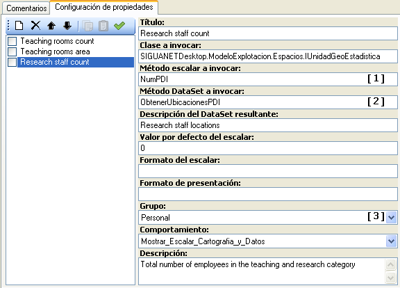
Key aspects in this measurement:

• [1] The NumPDI scalar method will return a count of teachers and researchers.
• [2] The ObtenerUbicacionesPDI collection method will return teaching and research employee locations.
• [3] The Staff category (Personal) is assigned so that this measurement doesn't get mixed with measurements in the Enclosures category.

When dealing with work places, occupancy rates may be also relevant. If you want to know how many square meters are available per research employee and the variation of this rate across different levels of spatial aggregation, this is how to do it:

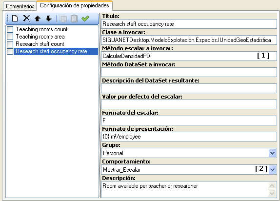
From the image above, you should have noticed this measurement definition is somewhat different:

• [1] There's a CalcularDensidadPDI scalar method that will return the occupancy rate, but there's no collection method. You'll find a section on rate calculation methods in the Appendix A: The IUnidadGeoEstadistica interface page.
• [2] Since we only need to display the scalar output of this measurement and a detail view won't be shown, the Mostrar_Escalar behaviour is selected.

And finally, what about teaching and research employees whose location is still unknown by the system? Everyone in your SIGUANET database must have a location, that is, an employee cannot be assigned a null enclosure identifier. This may cause problems since someone's location may not be known at the moment of inserting the record or just because there is an update from which we can infer a change in location but it cannot be precisely determined (e.g. a department transfer). To solve this there's a SIGUANET convention: use a fake enclosure whose identifier is

0000PB997

Whenever someone's assigned this identifier, it means location is pending. The siguanet_quest extension relies on this convention. So, here's how you can define a measurement on how many teachers or researchers are still waiting for a proper location in your SIGUANET database: