Exporting data from an epmGrid
On this page:
Link back to the table of contents.
A number of other R packages exist that perform operations on species communities. Probably the most common format for such data is a site by species presence/absence matrix.
It is possible to export information from an epmGrid object to this format with the function epmToPhyloComm().
You can either get specific sites by providing a set of coordinates, or you can get all sites (= all grid cells).
In the following example, we want to create such a presence/absence matrix for a specific set of sites. The epmGrid object is in an equal area projection, but we have our site coordinates in longitude/latitude. We will first need to transform these unprojected coordinates to the appropriate coordinate system.
> library(sf)
> # get the projection of the epmGrid object
> proj <- attributes(squirrelEPM)$crs
>
> # define some points in long/lat
> pts <- rbind.data.frame(
+ 		c(-120.5, 38.82),
+ 		c(-84.02, 42.75),
+ 		c(-117.95, 55.53))
> colnames(pts) <- c('x', 'y')
>
> pts
        x     y
1 -120.50 38.82
2  -84.02 42.75
3 -117.95 55.53
>
> ptsSF <- st_as_sf(pts, coords = 1:2, crs = "epsg:4326")
> pts <- st_coordinates(st_transform(ptsSF, crs = proj))
>
> epmToPhyloComm(squirrelEPM, pts)
      Callospermophilus_lateralis Glaucomys_sabrinus Glaucomys_volans Marmota_monax
site1                           1                  1                0             0
site2                           0                  1                0             1
site3                           0                  1                1             1
      Otospermophilus_beecheyi Sciurus_carolinensis Sciurus_griseus Sciurus_niger
site1                        1                    0               1             0
site2                        0                    0               0             0
site3                        0                    1               0             1
      Tamias_amoenus Tamias_minimus Tamias_quadrimaculatus Tamias_senex
site1              1              1                      1            1
site2              0              1                      0            0
site3              0              0                      0            0
      Tamias_speciosus Tamias_striatus Tamiasciurus_douglasii Tamiasciurus_hudsonicus
site1                1               0                      1                       0
site2                0               0                      0                       1
site3                0               1                      0                       1
A common task might be to calculate diversity metrics and to then perform statistical analyses to investigate potential relationships between diversity metrics, and/or with other types of data.
The function tableFromEpmGrid() will generate the sort of data typically needed for such statistical analyses.
In a nutshell, given a set of locations (either all grid cells, specific coordinates, or a random subsample of grid cells), the function will return the values found at those locations for all inputs.
Inputs can be a mix of epmGrid objects, polygons with data attributes, or raster datasets.
For example, let's say we are interested in exploring the relationship between species richness, morphological shape disparity, phylogenetic diversity and topographic ruggedness.
First, let's generate those diversity metrics:
library(epm)
library(sf)
library(terra)

morphDisp <- gridMetrics(squirrelEPM, metric = 'disparity')
pd <- gridMetrics(squirrelEPM, metric = 'pd')
Now we will load an elevation dataset (this one for example)[https://www.usgs.gov/coastal-changes-and-impacts/gmted2010].
> elev <- rast('~/Dropbox/elev_GMTED2010.tif')
> elev
class       : SpatRaster
dimensions  : 20880, 43200, 1  (nrow, ncol, nlyr)
resolution  : 0.008333333, 0.008333333  (x, y)
extent      : -180.0001, 179.9999, -90.00014, 83.99986  (xmin, xmax, ymin, ymax)
coord. ref. : lon/lat WGS 84 (EPSG:4326)
source      : elev_GMTED2010.tif
name        : elev_GMTED2010
min value   :           -430
max value   :           8625
The elevation raster is unprojected, has a global extent, and has a resolution of ~ 1km (30 arc-seconds). We will therefore crop it to the extent of our epmGrids, and we will also need to project it to the coordinate system of our epmGrids.
elevCropped <- crop(elev, vect(st_transform(squirrelEPM[[1]], crs = 4326)))
elevCroppedEA <- project(elevCropped, attributes(squirrelEPM)$crs)
topoComplexity <- terrain(elevCroppedEA, v = 'TRI')
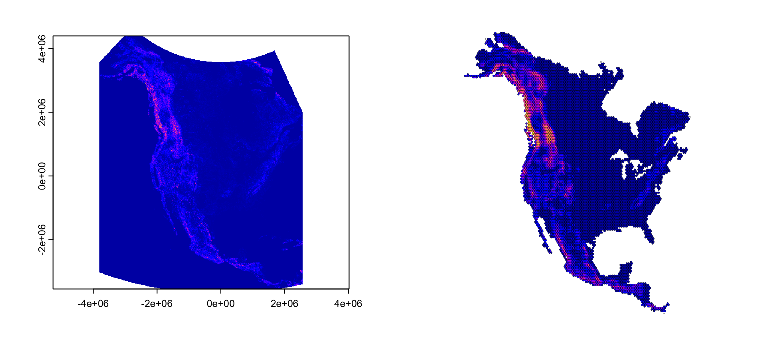
Here, we could pass the raster topoComplexity to the tableFromEpmGrid() function. What would happen then is grid cell centroids from across our epmGrid objects would be used to extract data from this raster. But this means that we will get the topographic complexity at the 1km x 1km raster cell that aligns with the center of the epmGrid cell that is at 50km resolution. Is that raster cell a good representation of the area encompassed by the larger epmGrid grid cell?
It depends! It might not be. Maybe it would make more sense to get the average of those higher resolution raster cells that overlap with the epmGrid grid cell. The function rasterToGrid() does exactly this. Given a raster object and a target grid that should be matched (such as a epmGrid object), the function will return a new grid that has the same spatial properties as the target grid, but where values are averages from the original grid.
topoComplexityPoly <- rasterToGrid(topoComplexity, squirrelEPM)

plot(topoComplexity, xlim = st_bbox(squirrelEPM[[1]])[c(1,3)], ylim = st_bbox(squirrelEPM[[1]])[c(2,4)], col = sf.colors(100), legend = FALSE)
plot(topoComplexityPoly, reset = FALSE, key.pos = NULL, lwd = 0.25, main = NULL)
Now let's run the epm function:
xx <- tableFromEpmGrid(squirrelEPM, morphDisp, pd, topoComplexityPoly, n = 1000)
The column headers are pulled from the input data, but may not always be informative. We'll replace them.
> colnames(xx) <- c('x', 'y', 'richness', 'disparity', 'pd', 'topoComplexity')
> head(xx)
         x         y richness   disparity        pd topoComplexity
1 -3083291 4191033.3        2 0.018304045  67.59251      1.5093903
2  -608291 -442202.6        3 0.004399944  53.05319      4.5886161
3   391709 1809463.5        4 0.010541032 117.33541      0.9873409
4 -1483291 -572106.4        3 0.002372681  62.35155     11.0377967
5 -1083291 1419752.0        3 0.010836528  92.04679      9.3543581
6   991709 -702010.2        6 0.007008325 142.50335      6.5881442

> dim(xx)
[1] 1000    6
It might be desirable to retain the coordinates for use in a complementary analysis, or to make this repeatable. You can save the coordinates (write them to a file), and then supply them to the tableFromEpmGrid function.
sampleCoords <- as.matrix(xx[,1:2])
xx2 <- tableFromEpmGrid(squirrelEPM, morphDisp, pd, topoComplexityPoly, coords = sampleCoords)
From, here we could run spatial autoregressive models, GAM's or other statistical approaches that account for spatial autocorrelation.