get_started
Welcome to Sequential_Fish get started section. This section will help you learn how to set up your working directory and launch your first quantification.
While functioning and to output quantification and analysis results the pipeline will write files to your disk. Everything will be stored in the working directory. Each dataset you process should have its own working directory.
Here is the typical and minimal required file structure to run a quantification.
In this example folder we find the FISH_STACK folder containing one subfolder for each field of view acquired.
Note that each location folders contains the images stack as ome.tiff.
The experience_file.xlsx contains the information on your experiment cycle order.
working_directory
├── experience_file.xlsx
└── FISH_STACK
    ├── Location01
    │   ├── img000_000_000000_0000000000.ome.tiff
    │   ├── img000_000_000000_0000000000.ome.tiff
    │   ├── img000_000_000000_0000000000.ome.tiff
    │   ├── img000_000_000000_0000000000.ome.tiff
    │   ├── img000_000_000000_0000000000.ome.tiff
    │   └── ...
    ├── Location02
    │   ├── img000_000_000000_0000000000.ome.tiff
    │   ├── img000_000_000000_0000000000.ome.tiff
    │   ├── img000_000_000000_0000000000.ome.tiff
    │   ├── img000_000_000000_0000000000.ome.tiff
    │   ├── img000_000_000000_0000000000.ome.tiff
    │   └── ...
    ├── Location03
    │   ├── img000_000_000000_0000000000.ome.tiff
    │   ├── img000_000_000000_0000000000.ome.tiff
    │   ├── img000_000_000000_0000000000.ome.tiff
    │   ├── img000_000_000000_0000000000.ome.tiff
    │   ├── img000_000_000000_0000000000.ome.tiff
    │   └── ...
    ...
The experience file contains the information on the fluidics cycle. It should contains one line per cycle and one column per acquisition channel.
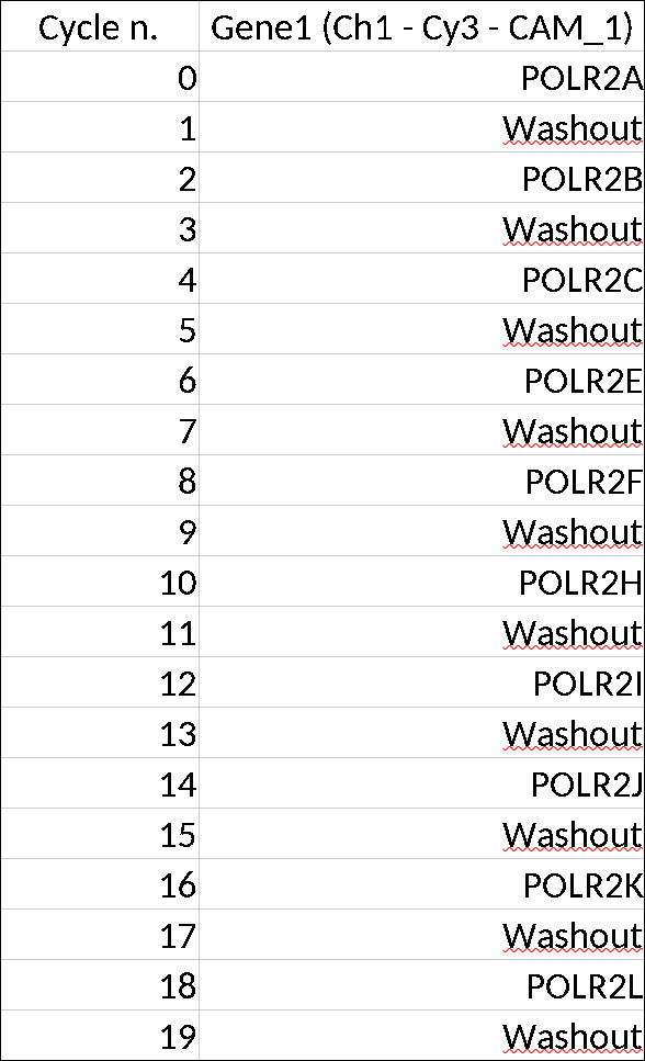
Note that washout cycles are specified with same name wheras interest genes should have different names in each cycles.
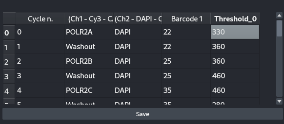
Later on we will add an other column to the file containg the thresholds used for single molecule detection. But first we need to set-up the pipeline parameters.
Now you have set up the working directory we need to configure the pipeline settings. This will create a pipeline_parameters.json file in your working directory so you can set up different parameters for different experiments with no risk to mix them up.
Open a terminal and activate your Sequential_Fish environnement then run the command :
(Sequential_Fish) python -m Sequential_Fish settings pipeline "path_to_working_directory"This command will inizialise your pipeline_parameters.json and prompt you with a graphical interface to set parameters. For now let us at the general tab containing all parameters needed to run the input step of pipeline.
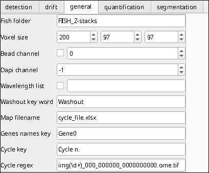
- Fish folder : Folder containing all the location folder as mentionned above.
- Voxel Size : (zyx) Size of pixel from your microscope in nanometers, z size corresponds to the distance between two slices.
- Bead channel : depreciated
- Dapi channel : Index of channel containing dapi signal, starting from 0 : channel 1 is indexed 0. If last channel you can leave -1.
- Wavelength list : If imaging single molecules in several colors, tick the box and indicate in order corresponding wavelength in nanometers delimited by commas. (i.e) 555,640 .
- Washout key word : Key word to recognize washout cycles, this is the same keyword that should be written in the experience file.
- Map filename : Filename of the experience file including file extension.
- Genes names key : List of all columns names in the experience file containing genes to detect. Use commas to delimit two columns.
- Cycle key : Name of column indicating cycles in the experience file.
- Cycle regex : Regex capturing the filename of image stacks. There should be a capturing group (i.e parenthensis) capturing cycle number.
Here are the settings filled with the information from our example working directory. Note that wavelength list is not filled as we have only one imaging channel. In this example FISH signal is in channel 1 (indexed 0) and DAPI signal is in channel 2 (indexed 1).
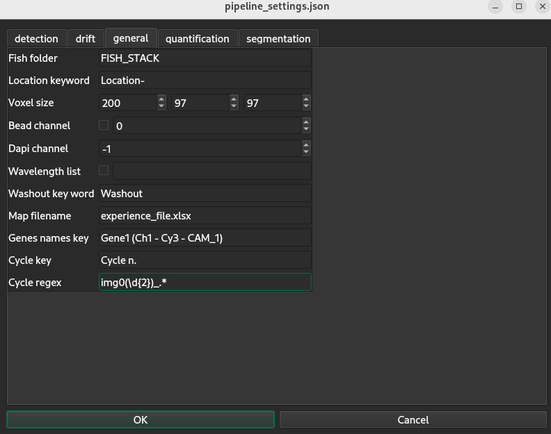
Click OK to validate your input. A new file pipeline_parameters.json is created (or updated) in your working directory. Next step is to run the input step from the quantification pipeline.
About regex
Regex are designed to to capture information from a string (text) in order to do so it describes a way to match a sequence of caracter here img0(\d{2})_. * will match sequences starting with img0 then followed by two integers then followed by _ and any caracter afterwards.
Note that the parenthesis () are delimiting the capturing group in other word the information we want to extract from the sequence, so in this case the two integers (\d{2}) which correspond to the cycle number. You can learn more about this and test your regex on regexr website.
The input step is the basis of Sequential Fish package and should be run before anything else. It allows the software to map your working directory and every cycles and locations in your image stacks. To launch it type the following command in your terminal :
(Sequential_Fish) python -m Sequential_Fish pipeline input "path_to_working_directory"A detailed description of the input step is available in this section. To sum up the software will assign each cycle to corresponding genes and map every locations you have imaged, This information is stored in the result_tables/ folder inside two tables : Input and Gene_map. Additionaly, the input script will check correct the structure of the working directory and that mapping matches information found in the images stack. You can follow input processing in the terminal, if any error should occur they will be written in the run_log.log file at the root of your working directory.
From there we can start to quantifify our data they are several ways to process forward, to better understand what will happen to your data let us open the viewer module.
We will now perform interactive single molecule detection and cell segmentation to better understand the parameters you will have to set. To this end we open the viewer module by running the command :
(Sequential_Fish) python -m Sequential_Fish viewer "path_to_working_directory"
If you already used napari before you can notice a few widgets are have been added to the interface. Upon opening you should see on the right the Data enabled allowing us to load data. Before clicking anything let us notice the other two tabs : Segmentation and Thresholds as well as the select locations button on the bottom left corner of the screen. When performing action in the viewer such as loading visual data the software will load the data for all selected locations which can be time consuming and memory intensive. For now, for a better interactivity let us select one location from the pannel and click the select locations button. Then on the right pannel select a target you would like to visualize, in my case, POLR2A and then click the load signal button.
Tip : While using the napari viewer keep an eye on the terminal window which will inform you of actions progression.
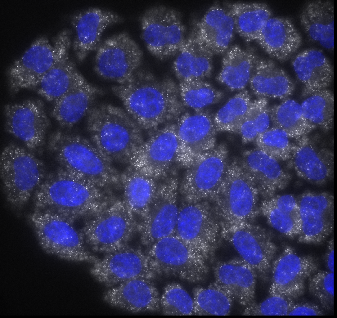
After loading your image you can modify some visualization options such as the contrast and the colormap. Now for segmentation purpose let us visualize also the dapi. Without changing the target tick the dapi radio button and again load signal button. By default dapi is loading in blue but again you can change colormap and contrast if needed.
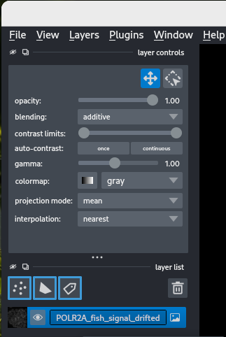
To beging let us select the Segmentation tab on the bottom right of the interface. This will show the segmentation widget using cellpose cpsam model. For our first try let us try to segment nuclei out of the box. In the image parameter select the layer which name contains dapi_signal and click the Run button.
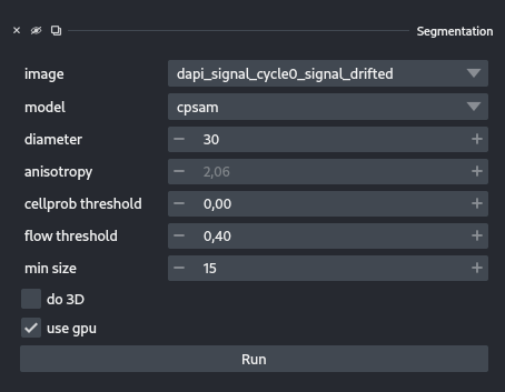
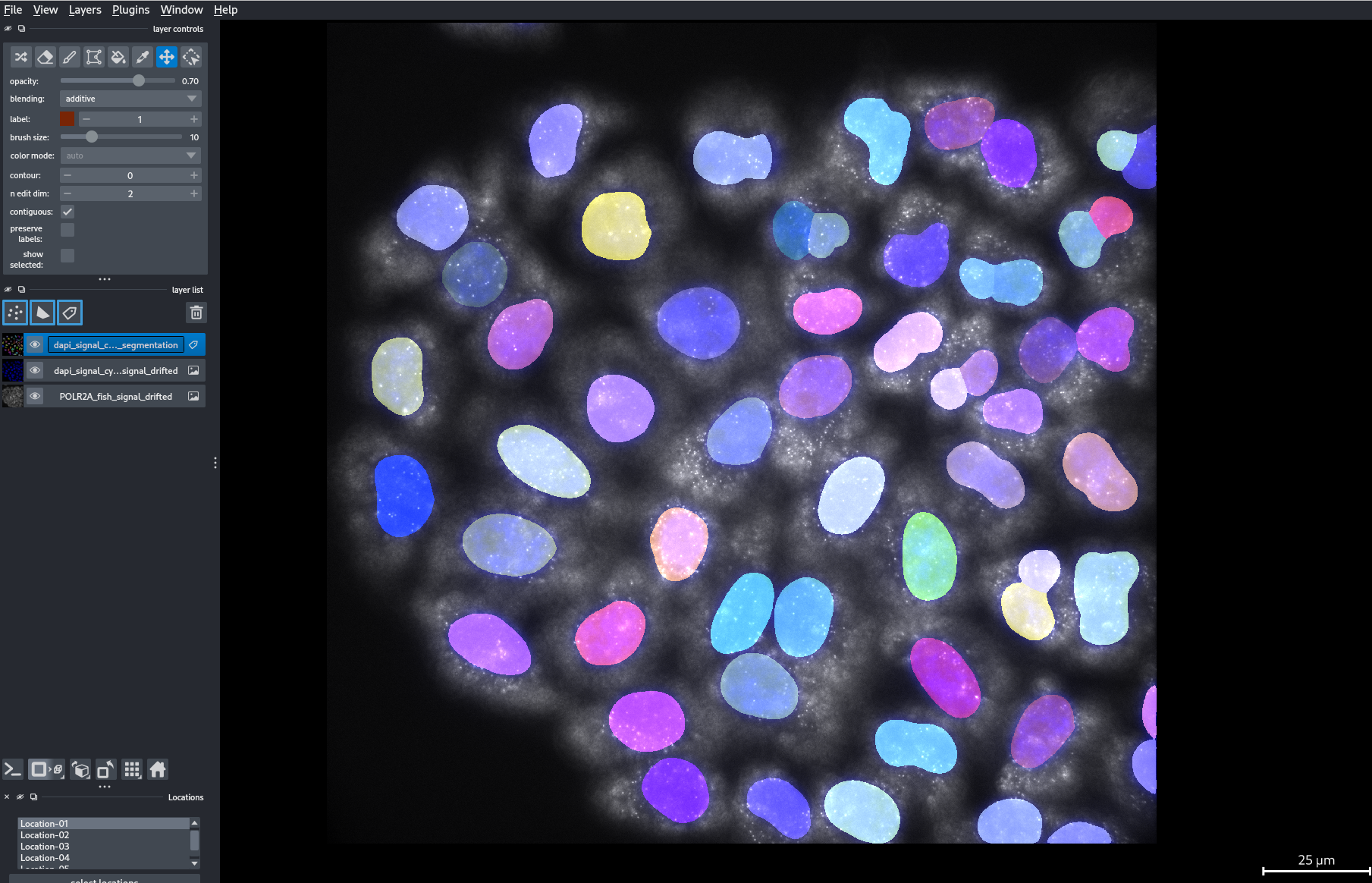
Here is your first segmentation ! Now you can try for yourself to play with the different cellpose paramters or to try 3D segmentation. Firstly, I recommend to play around with the diameter paramter that has a huge impact on segmentation. On the worst case scenario cellpose also offer the possibility to retrain models for better results.
Once statisfied with your parameters for both nuclei and cytoplasm segmentation we can enter them in the settings. To that end run the command in your terminal (after closing napari or by opening another terminal) and click the segmentation tab.
(Sequential_Fish) python -m Sequential_Fish settings pipeline "path_to_working_directory"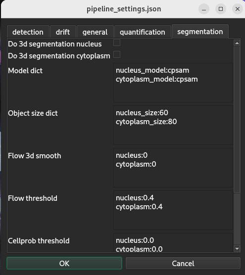
This section aims to get your started with single molecule detection and threshold setting. For a full insight on algorithm functionment checkout the dedicated section.
First open the viewer and load a fish signal as described above and go in the Thresholds tab in the bottom right corner of the interface.
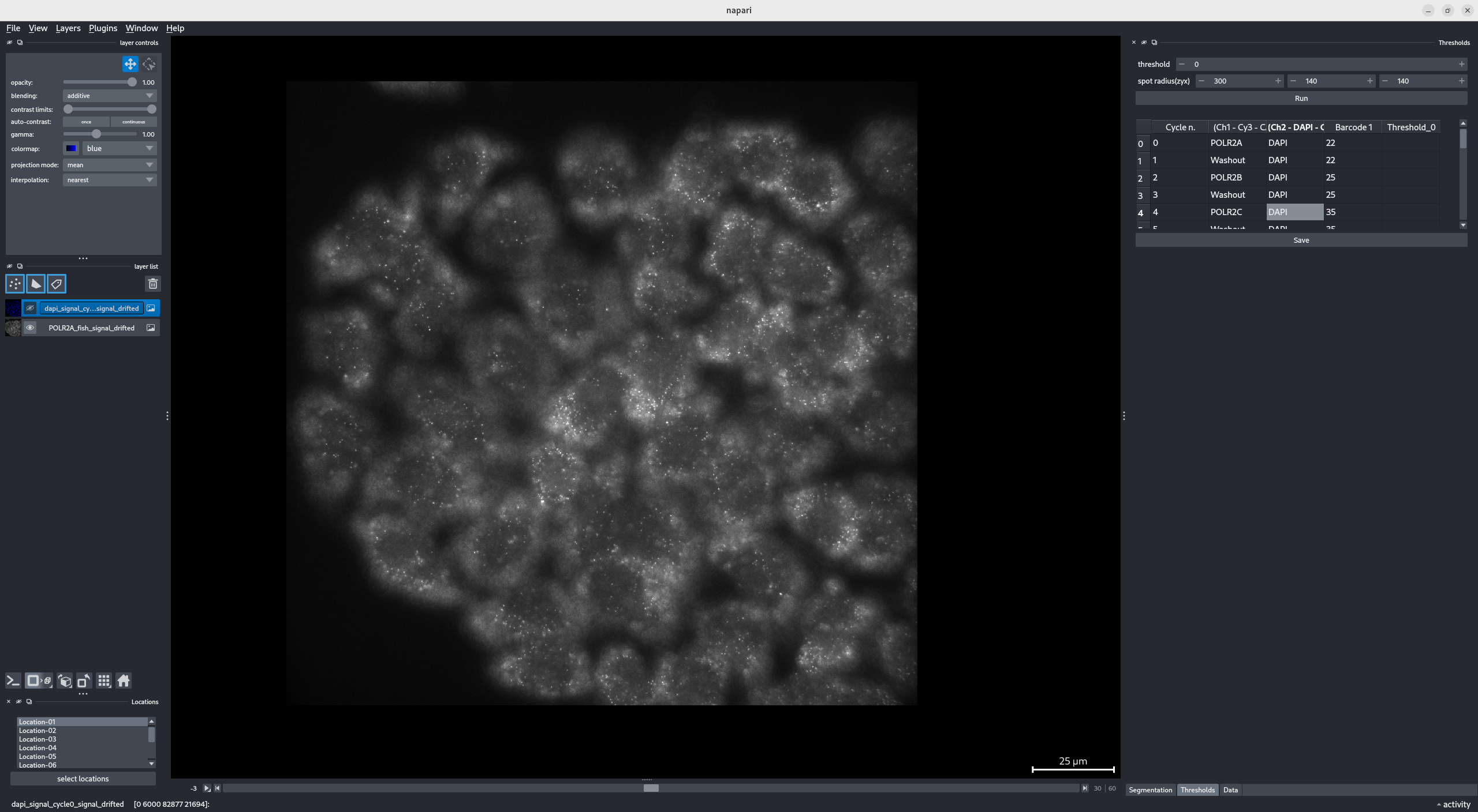
To perform detection you will have to set a threshold for each cycle and for each color. The value of the threshold will be strongly signal dependent, to get and understanding of the detection process let us try with a threshold set to 100. Enter 100 in the threshold value in the top right corner leave the spot size for now. Note that the spot size is set to 1.5x your voxel size parameter by default. Select your FISH layer by clicking it on the left panel and click the Run button.
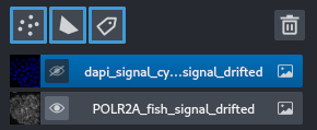
Hide a layer : You can hide a a layer on the left pannel by clicking the eye icon next to its name. In the screenshot above I hid the dapi layer.
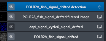
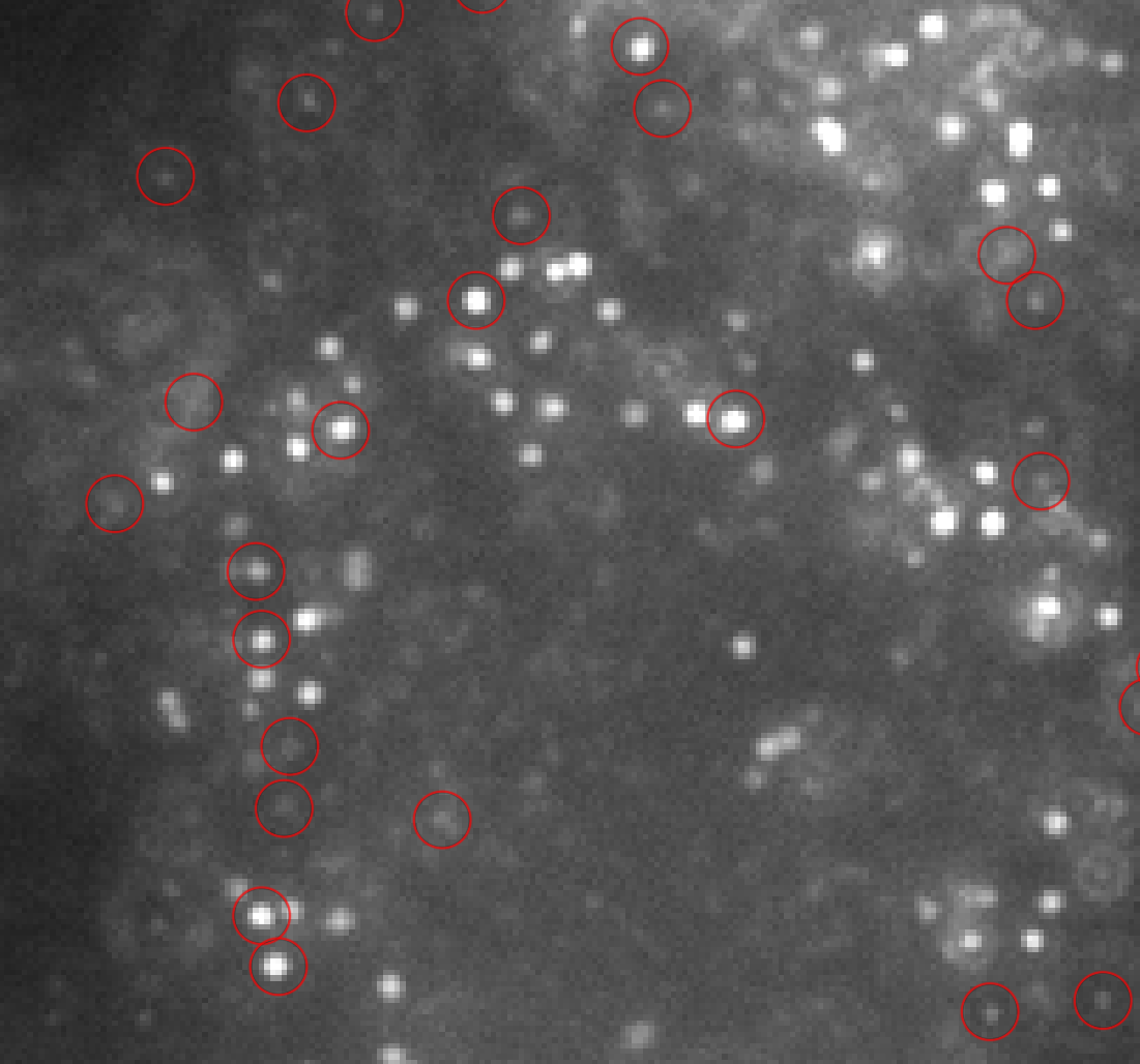
Two new layers are added to the viewer : filtered image a signal layer and detection a point layer.
-
The detection layer shows were the single molecule were detected with red circles. Looking at the above screenshot you will notice that most bright spot were not detected but remember that spot detection is performed in 3D in my case all bright spots were detected at other z level. However, we can also see that false spot were detected indicating a threshold too low.
-
The filtered image layer is an enhanced image for spot detection it is computed on original signal using a Laplacian of Gaussian filter (LoG). The thresholds are set as cutoffs for the values of the filtered image and not the original signal.
Setting thresholds is the most time consuming step for user as you will have to process through tries and repeats to find an apropriate threshold for each cycle and each color. The purpose of this section is just to get you started with spot detection but you can find my complete process for setting a threshold in the detection section.
Reading pixel value
To read a pixel value on Napari first select the layer from which you want the value and then hover the pixel of interest. You will be able to read the value on the bottom left corner.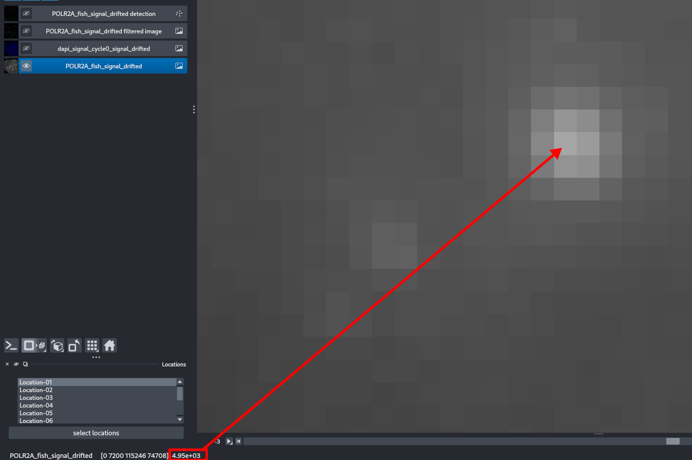

When reaching a satisfying threshold value enter it in the appropriate column in the table on the right and click the save button, this will update your experience file. Once all the thresholds are completed you are ready to launch the pipeline ! If you modified the spot size don't forget to update your pipalne parameters.
You are ready to launch the pipeline, enter the command below to start. You can monitor progress directly or in the run_log.log file located at your working directory's root.
Computation will take several hours depending on your configuration, dataset and parameters, in the meantime you can read more about the pipeline or about the analysis. In case you run into any issue and have to reload the pipeline you don't have to reload from start, checkout the command line section. If you are blocked or spot any unintended behavior consider opening an issue on the github.
(Sequential_Fish) python -m Sequential_Fish pipeline "path_to_working_directory"Upon progression in the pipeline a lot more tools will be enabled to monitor quantification in the viewer module, a full documentation is available here.