Basic Tutorials
A simple page and file set that allows you to test the basic operations of NAS6LIB in the console.
It also includes minimal integration samples with 3D rendering libraries such as Three.js and X3DOM.
Please enable comments and add test code to make use of it.
TestPage ZipFile (External Link)
testpage000 DEMO (External Link)
test3JS000 DEMO (External Link)
testX3DOM000 DEMO (External Link)
NAS6LIB has no dependencies on other existing libraries.
NAS6LIB is designed to be used almost standalone, but it can be used more conveniently
when used in conjunction with JQuery property access, X3DOM, and ThreeJS's advanced rendering functions.
As shown in Minimal tutorial
*.js files for each module of NAS6LIB can be used by loading external files using script tags.
Please scroll up a little to see the project template.
-
Quick Start
- 1. Load the Library
Include the necessary JavaScript files in your HTML.
Add other modules like vector.js, matrix.js, quaternion.js, planet.js, etc.,
as needed for your specific use case.
HTML
<script src="https://nas6mixfoolv.github.io/NAS6LIB/javascripts/nas6lib/vector.js"></script>
-
2. Minimum Sample (2D Vector Addition)
Here's a simple JavaScript example to get started:
JavaScript
var v1 = new N6LVector([1, 2]);
var v2 = new N6LVector([3, 4]);
var v3 = v1.Add(v2);
console.log(v3.x); // Result: [4, 6]
Loading the Library
HTML
<script src="https://nas6mixfoolv.github.io/NAS6LIB/javascripts/nas6lib/vector.js"></script>
<script src="https://nas6mixfoolv.github.io/NAS6LIB/javascripts/nas6lib/matrix.js"></script>
<script src="https://nas6mixfoolv.github.io/NAS6LIB/javascripts/nas6lib/quaternion.js"></script>
elements order is w-x-y-z-...
JavaScript
//Fourth-order vector
var veca = new N6LVector(4);
//Homo fourth-order vector
var vecb = new N6LVector(4, true);
//Third-order vector
var vecc = new N6LVector(new Array(1, 2, 3));
//x-axis unit homo fourth-order vector
var vecd = new N6LVector(new Array(1, 1, 0, 0), true);
var vece = new N6LVector([1, 1, 0, 0], true);
var vecf = new N6LVector(4, true).UnitVec(1);
//zero homo fourth-order vector
var vecg = new N6LVector(new Array(1, 0, 0, 0), true);
var vech = new N6LVector([1, 0, 0, 0], true);
var veci = new N6LVector(4, true).ZeroVec();
//deep copy
var vecf = new N6LVector(veci);

//4 rows and 4 columns
var mata = new N6LMatrix(4);
//4 rows and 8 columns
var matb = new N6LMatrix(4, 8);
//4 rows and 4 columns unit matrix
var matc = new N6LMatrix(new Array(1, 0, 0, 0, 0, 1, 0, 0, 0, 0, 1, 0, 0, 0, 0, 1), 4, 4);
var matd = new N6LMatrix(new Array(
      new N6LVector(new Array(1, 0, 0, 0)),
      new N6LVector(new Array(0, 1, 0, 0)),
      new N6LVector(new Array(0, 0, 1, 0)),
     new N6LVector(new Array(0, 0, 0, 1)) ));
var mate = new N6LMatrix([[1, 0, 0, 0], [0, 1, 0, 0], [0, 0, 1, 0], [0, 0, 0, 1]] );
//deep copy
var matf = new N6LMatrix(mate);
/*
note:Fourth-order or more is considered to be a homogeneous coordinates
If you want to make a fourth-order or more conventional coordinate N6LMatrix.SetHomo(false)**
Please continue to build declaration
*/
* Addition, subtraction, multiplication (vectors and matrices, matrices and matrices), Division (for convenience)
JavaScript
//Vector
/*
When bHomo=true, the w element is skipped.
*/

//[1, 2] + [3, 4] = [4, 6]
var v1 = new N6LVector([1, 2]);
var v2 = new N6LVector([3, 4]);
var v3 = v1.Add(v2);
console.log(v3.x); // Result: [4, 6]
//[1, 2] + 3 = [4, 5]
var v4 = v1.Add(3);
console.log(v4.x); // Result: [4, 5]

//[3, 4] - [1, 2] = [2, 2]
var v5 = v2.Sub(v1);
console.log(v5.x); // Result: [2, 2]
//[3, 4] - 2 = [1, 2]
var v6 = v2.Sub(2);
console.log(v6.x); // Result: [1, 2]

//[1, 2] * [3, 4] = 11
var n1 = v1.Mul(v2);
console.log(n1); // Result: 11
//[1, 2] * [[1, 2], [3, 4]] = [7, 10]
var m1 = new N6LMatrix([[1, 2], [3, 4]]);
var v7 = v1.Mul(m1);
console.log(v7.x); // Result: [7, 10]
//[1, 2] * 2 = [2, 4]
var v8 = v1.Mul(2);
console.log(v8.x); // Result: [2, 4]

//[3, 4] / [1, 2] = 5
var n2 = v2.Div(v1);
console.log(n2); // Result: 5
//[3, 4] / [[1, 2], [3, 4]] = [4.333..., 2.5]
var v9 = v2.Div(m1);
console.log(v9.x); // Result: [4.333..., 2.5]
//[3, 4] / 2 = [1.5, 2]
var v10 = v2.Div(2);
console.log(v10.x); // Result: [1.5, 2]

//Matrix

//[[1, 2], [3, 4]] + [[2, 4], [6, 8]] = [[3, 6], [9, 12]]
var m2 = new N6LMatrix([[2, 4], [6, 8]]);
var m3 = m1.Add(m2);
console.log(m3.x); // Result: [[3, 6], [9, 12]]
//[[1, 2], [3, 4]] + 2 = [[3, 4], [5, 6]]
var m4 = m1.Add(2);
console.log(m4.x); // Result: [[3, 4], [5, 6]]

//[[2, 4], [6, 8]] - [[1, 2], [3, 4]] = [[1, 2], [3, 4]]
var m5 = m2.Sub(m1);
console.log(m5.x); // Result: [[1, 2], [3, 4]]
//[[2, 4], [6, 8]] - 1 = [[1, 3], [5, 7]]
var m6 = m2.Sub(1);
console.log(m6.x); // Result: [[1, 3], [5, 7]]

//[[1, 2], [3, 4]] * [[2, 4], [6, 8]] = [[14, 20], [30, 44]]
var m7 = m1.Mul(m2);
console.log(m7.x); // Result: [[14, 20], [30, 44]]
//[[1, 2], [3, 4]] * [1, 2] = [5, 11]
var v11 = m1.Mul(v1);
console.log(v11.x); // Result: [5, 11]
//[[1, 2], [3, 4]] * 2 = [[2, 4], [6, 8]]
var m8 = m1.Mul(2);
console.log(m8.x); // Result: [[2, 4], [6, 8]]

//[[2, 4], [6, 8]] / [[1, 2], [3, 4]] = [[3.333..., 2], [8.666..., 5]]
var m9 = m2.Div(m1);
console.log(m9.x); // Result: [[3.333..., 2], [8.666..., 5]]
//[[2, 4], [6, 8]] / [1, 2] = [4, 10]
var v12 = m2.Div(v1);
console.log(v12.x); // Result: [4, 10]
//[[2, 4], [6, 8]] / 2 = [[1, 2], [3, 4]]
var m10 = m2.Div(2);
console.log(m10.x); // Result: [[1, 2], [3, 4]] JavaScript
//Vector

//[3, 4].Abs() = 5
var v1 = new N6LVector([3, 4]);
var n1 = v1.Abs();
console.log(n1); // Result: 5
//[3, 4].Normal() = [3/5=0.6, 4/5=0.8]
var v2 = v1.NormalVec();
console.log(v2.x); // Result: [3/5=0.6, 4/5=0.8]
//[3, 4].Normal([6, 8]) = [3/5=0.6, 4/5=0.8]
var v3 = new N6LVector([6, 8]);
var v4 = v1.NormalVec(v3);
console.log(v4.x); // Result: [3/5=0.6, 4/5=0.8]

//Matrix

//[[2, 0], [0, 2]].Normal() = [[1, 0], [0, 1]]
var m1 = new N6LMatrix([[2, 0], [0, 2]]);
var m2 = m1.NormalMat();
console.log(m2.x); // Result: [[1, 0], [0, 1]]JavaScript
//Vector

//[3, 4].Dot([5, 6]) = 3*5+4*6=39
var v1 = new N6LVector([3, 4]);
var v2 = new N6LVector([5, 6]);
var n1 = v1.Dot(v2);
console.log(n1); // Result: 3*5+4*6=39
//[3, 4].Cross([5, 6]) = 3*6-4*5=-2
var n2 = v1.Cross(v2);
console.log(n2); // Result: 3*6-4*5=-2JavaScript
//Matrix

//[[1, 0, 0, 0], [2, 0, 0, 1], [3, 0, 1, 0], [4, -1, 0, 0]].Transpose() = [[1, 2, 3, 4], [0, 0, 0, -1], [0, 0, 1, 0], [0, 1, 0, 0]]
//[[1, 0, 0, 0], [2, 0, 0, 1], [3, 0, 1, 0], [4, -1, 0, 0]].Inverse() = [[1, 0, 0, 0], [2, 0, 0, -1], [3, 0, 1, 0], [4, 1, 0, 0]]
var m1 = new N6LMatrix([[1, 0, 0, 0], [2, 0, 0, 1], [3, 0, 1, 0], [4, -1, 0, 0]]);
var m2 = m1.TransposedMat();
console.log(m2.x); // Result: [[1, 2, 3, 4], [0, 0, 0, -1], [0, 0, 1, 0], [0, 1, 0, 0]]
var dt = [];
var m3 = m1.InverseMat(dt);
console.log(m3.x); // Result: [[1, 0, 0, 0], [2, 0, 0, -1], [3, 0, 1, 0], [4, 1, 0, 0]]


//[[0, 0, 1], [0, 1, 0], [-1, 0, 0]].Transpose() = [[0, 0, -1], [0, 1, 0], [1, 0, 0]]
//[[0, 0, 1], [0, 1, 0], [-1, 0, 0]].Inverse() = [[0, 0, -1], [0, 1, 0], [1, 0, 0]]
var m4 = new N6LMatrix([[0, 0, 1], [0, 1, 0], [-1, 0, 0]]);
var m5 = m4.TransposedMat();
console.log(m5.x); // Result: [[0, 0, -1], [0, 1, 0], [1, 0, 0]]
var m6 = m4.InverseMat(dt);
console.log(m6.x); // Result: [[0, 0, -1], [0, 1, 0], [1, 0, 0]]JavaScript
//Matrix

//[[1, 0, 0, 0], [0, 1, 0, 0], [0, 0, 1, 0], [0, 0, 0, 1]].Translate([1, 2, 3, 4]) = [[1, 0, 0, 0], [2, 1, 0, 0], [3, 0, 1, 0], [4, 0, 0, 1]]
var m1 = new N6LMatrix(4).UnitMat();
var v1 = new N6LVector([1, 2, 3, 4], true);
var m2 = m1.TranslatedMat(v1);
console.log(m2.x); // Result: [[1, 0, 0, 0], [2, 1, 0, 0], [3, 0, 1, 0], [4, 0, 0, 1]]JavaScript
//Matrix

var m1 = new N6LMatrix(4).UnitMat();
var v2 = new N6LVector([Math.PI / 2.0, 0, 1, 0], true);
var v3 = new N6LVector([1, 2, 2, 2],true);
var v4 = new N6LVector([1, 3, 4, 5],true);
var m3 = m1.AffineMat(v3, v2, v4);
console.log(m3.x); // Result: [[1, 0, 0, 0], [3, 0, 0, 2], [4, 0, 2, 0], [5, -2, 0, 0]]
var v5 = new N6LVector([1, 0, 1, 0], true);
var m4 = m3.RotAxis(v5, -Math.PI / 2.0);
console.log(m4.x); // Result: [[1, 0, 0, 0], [3, 2, 0, 0], [4, 0, 2, 0], [5, 0, 0, 2]]JavaScript
//Local & World

//Matrix
var um = new N6LMatrix(4).UnitMat();
var ay = new N6LVector(4, true).UnitVec(2);
var lm1 = um.RotAxis(ay, Math.PI / 2.0);
var tr = new N6LVector([1, 0, 0, 5], true);
var lm2 = lm1.TranslatedMat(tr);
console.log(lm2.x); // Result: Local[[1, 0, 0, 0], [0, 0, 0, 1], [0, 0, 1, 0], [5, -1, 0, 0]]
var lm3 = lm2.TranslatedMat(tr.Mul(-1));
var lm4 = lm3.RotAxis(ay, -Math.PI / 2.0);
console.log(lm4.x); // Result: World[[1, 0, 0, 0], [0, 1, 0, 0], [0, 0, 1, 0], [0, 0, 0, 1]]NAS6LIB uses row-major matrix arrangement,
but many renderers use column-major matrix arrangement.
Also noteworthy is that a vector or matrix acting as the left operand is multiplied
by a vector or matrix acting as the right operand. This comes from the experience of
operator overloading in C# managed code, and comes from the programming convention of
calling a member function from the class entity of the left operand.
Note:
In NAS6LIB,
N6LVector.Mul(N6LVector or N6LMatrix etc = rh)
N6LMatrix.Mul(N6LVector or N6LMatrix etc = rh),
lh uses the stored row vector as is,
but rh takes the column vector obtained after transposing
and implements the multiplication of those vectors.
I will explain the differences in their calculation applications.
There are row-major and column-major arrangements for rotation matrices.
To explain it simply,
row-major arrangement means that each local axis is arranged by row,
column-major arrangement means that each local axis is arranged by column.
And mathematically, vector multiplication by a matrix is determined as follows:
(each element of the row of a vector or matrix) x (each element of the column of a vector or matrix).
This also involves the discussion of the world system and the view system.
By mathematical definition, the world system is untransformed, and the view system
is the inverse matrix of the world system, that is, the optimized transpose matrix.
To put it more simply, the world system and the view system are in an inverse relationship,
facing each other directly. If you place a figure on a desk facing you, if you are
in the view system coordinate system, the figure's coordinate system is the world coordinate system,
and if you are in the world system coordinate system, the figure's coordinate system is the view system.
The relationship between the signs of the local axes can be reversed. If you don't confirm this first,
you'll just end up talking the other way around.
Here I will explain from the perspective of the world, which is the opposite of the general view perspective.
When M is a regular matrix,
In other words,
Therefore,
if
In particular, for orthogonal matrices such as rotation matrices,
the inverse matrix is equal to the transpose matrix
the computational load of the transformation.
Here, the main calculations that the renderer performs are those
that are displayed on the final screen, so it is convenient to handle the (transposed) view system.
Going back to the definition of
(each element of a row in a vector or matrix) and (each element of a column in a vector or matrix),
if a matrix M is the left operand, that is, in the case of operations such as Mv and MN,
M is (each element of a row in a vector or matrix) and you multiply it by something,
so row-priority arrangement is convenient.
In other words, if you focus on M and consider its arrangement,
Row-priority arrangement:
Column-priority arrangement:
This is the story from the perspective of the world.
With this as a premise,
The reason that the renderer adopts column-priority instead of this is, as mentioned earlier,
because it is a calculation that is displayed on the final screen, it is a (transposed) view system.
Here's the story told by the view matrix.
Row-priority arrangement:
Column-priority arrangement:
This is a concept that is easily misunderstood, so please carefully consider the following.
Since the renderer is the calculation that is ultimately displayed on the screen,
it is convenient for a renderer that mainly handles the view matrix to mainly handle
but the reverse relationship is convenient when mainly handling the world matrix.
To put this simply, the renderer's main function is to calculate the view matrix,
so when viewed from the perspective of the world matrix,
the renderer's calculations are the transposed inverse matrix.
Here are the key "inverse relationships" in 3D graphics that often cause confusion:
-
View Matrix and World Matrix: The view matrix is the inverse of the world matrix,
which for orthogonal matrices (like rotation matrices) is equivalent to its transpose.-
Meaning of 1.: The view system and the world system are in an inverse, "face-to-face" relationship.
Imagine you place a figure on a desk facing you. If you are describing the scene from
the view system's perspective (your eye), the figure's coordinate system is the world coordinate system.
Conversely, if you define a scene from a world-frame perspective (a coordinate system specific to your desk),
then the world-frame perspective becomes the viewpoint frame, and your eye's coordinate system
becomes the world frame. The signs of the local axes can appear reversed depending on
which system you are currently considering. It's crucial to confirm which
perspective (world or view) is being discussed first,
otherwise, your understanding might be completely opposite.
-
Meaning of 1.: The view system and the world system are in an inverse, "face-to-face" relationship.
-
Left-Handed vs. Right-Handed Coordinate Systems: These systems have an inverse relationship,
particularly concerning the direction of the Z-axis. -
Order of Multiplication and Transposition: The order in which a vector or matrix is multiplied
by another matrix often involves a transpose relationship depending on the convention
(e.g., row-major vs. column-major, pre-multiplication vs. post-multiplication).
Note on NAS6LIB's Implementation:
In NAS6LIB, for operations like
N6LVector.Mul(N6LVector or N6LMatrix etc = rh) and
N6LMatrix.Mul(N6LVector or N6LMatrix etc = rh):
The left-hand operand (lh, the object calling the method) directly uses its stored row vectors.
The right-hand operand (rh) is internally transposed to obtain its column vectors before the multiplication.
The multiplication is then performed as a dot product between these vectors.
Considering these points, here is a simplified concept:
Forward transform:
↑ Explanations from the perspective of the developer/library user are mainly focused on world matrices.
Inverse transform:
↑ Explanations from the perspective of the renderer are mainly focused on view matrices.
Forward transform:
Inverse transform:
The difference between ROTA and ROTB lies in whether the multiplication of the argument
input against the main matrix is performed from the right (post-multiplication)
or from the left (pre-multiplication). The difference between forward and inverse transforms
is whether the output is calculated from the input (forward) or the input is inferred from the output (inverse).
Of these, the view matrix-based inverse transformation is convenient from the renderer's perspective,
while the world matrix-based forward transformation is convenient from the library user's perspective. T
hus, even though you can retrieve the world matrix for cameras or objects in both ThreeJS and X3DOM,
the APIs provided by renderers for matrix multiplication and other operations are still
often designed primarily for the view, not the world. Therefore, it's frequently more efficient
to calculate the inverse matrix (i.e., the transpose) and then transpose it again when necessary.
This understanding is extremely useful when creating programmable shaders.
The reason why the renderer adopts a column-major matrix arrangement is
inverse transformation: v(in) = ROTA^-1{ M^T v'(out) }
It is an inverse matrix, i.e. a transposed matrix, to be drawn on the screen as a view,
so if the arrangement is column-major, it will end up being row-major,
which is advantageous for two-dimensional arrays.
Furthermore, if we delve deeper into this discussion, we will inevitably arrive at the question of
why the direction of the cross product was determined to be left-handed or right-handed.
- Why is there a left-handed system when physics is all right-handed?
The horizontal axis of a graph is naturally left to right and the vertical axis
is naturally bottom to top, so to make the z-axis jump out of the plane, it is a right-handed system.
However, the vertical axis of a display plane, or text flow, is naturally top to bottom,
so this is a left-handed system. Also, as the medium for expressing characters shifted
from carving to writing, the order of text flow changed from right to left to left to right.
In other words, the direction of the axis is generally required by the change in the medium
for expressing it and the need for its direction.
In other words, in terms of graph, it is a right-handed system,
but in terms of text flow, the left-handed system can be conveniently expressed.
Also, an easy way to distinguish between right-handed and left-handed systems
is to fix the direction of the x-axis as left to right and the direction of the y-axis as bottom to top,
and a right-handed system is one in which the direction of the z-axis is from back to front,
and a left-handed system is one in which the direction of the z-axis is from front to back.
Note:
In 3DCG, you must first check whether you or someone else is talking
about the world matrix or the viewpoint matrix, otherwise you may end up
with a contradiction in perception, i.e. the opposite meaning.
note:
This is an explanation of homogeneous coordinates defined
in the order w, x, y, z, .... The order is different, but the function is the same...
Since NAS6LIB is not a renderer, there is no right-handed or left-handed system,
and it mainly follows the coordinate system of the renderer.
However, the cross product of vectors is defined in the right-handed system,
and as long as it follows the coordinate system of the renderer, no major problems will occur.
This section explains how N6L handles homogeneous coordinates and the significance of the bHomo flag,
which dictates special behaviors within the library.
-
Coordinate System Expectation
N6L is fundamentally based on DirectX's conventions, therefore, it expects a row-major, left-handed coordinate system.
It's important to note that if you're interacting with other libraries or APIs that adopt a right-handed coordinate system,
you might need to perform transformations like transposition or Z-axis inversion (multiplication by -1) during input and output.
However, as long as you're performing calculations purely within N6L, these external conversions aren't strictly necessary,
provided you consistently align your internal conventions.
- N6L's Matrix Layout
While homogeneous transformation matrices are typically represented as:
where ROT is the rotation component and T is the translation component, N6L adopts a slightly different,
though functionally equivalent, row-major layout for its internal representation. This specific arrangement does not cause any calculation issues.
N6L's expected matrix layout (row-major):
Mij is the rotational transformation component.
Tk is the translational component.
Row N0 is the w component row.
Row N1 is the row for the x-axis component of the rotation matrix (local coordinate system).
Row N2 is the row for the y-axis component of the rotation matrix (local coordinate system).
Row N3 is the row for the z-axis component of the rotation matrix (local coordinate system).
note:
Vector × matrix calculations are column-major calculations
Matrix × vector calculations are row-major calculations
The advantage of the row-major calculation format used by NAS6LIB
is that each axis of the local rotation transformation can be extracted straightforwardly as a row
The translation components in this case are arranged in columns
But by multiplying them with a homogeneous zero vector,
they can also be extracted straightforwardly
In this case, the row-major notation for the formula is mainly N6LMatrix.Mul(N6LVector),
but it is also possible to write it as column-major notation
N6LVector.Mul(N6LMatrix) depending on the situation.
Key Benefits of Homogeneous Coordinates
Using a homogeneous coordinate system and 4x4 matrices allows various 3D graphics transformations to be handled
as unified linear algebra operations. The benefits are immense:
-
Unified Transformation Representation:
-
Diverse transformations like translation, rotation, scaling, shearing, and even perspective projection
can all be expressed as a single 4x4 matrix multiplication. This simplifies complex transformation chains
(e.g., object rotation → translation → camera view transform) into straightforward matrix products,
significantly streamlining your code. Without homogeneous coordinates, different transformation types
would require distinct calculation methods, leading to much more complex code. -
Efficient Inverse Matrix Calculation (Especially for Rotation): You can extract the 3x3 rotation part from a 4x4 homogeneous matrix and leverage its orthogonal matrix properties
to find its inverse simply by transposing it. This optimization avoids computationally expensive general inverse matrix calculations
(like Gaussian elimination) and greatly contributes to real-time graphics performance. -
Perspective Projection Representation:
The w component of homogeneous coordinates is indispensable for representing perspective projection (depth perception).
As an object's distance changes, its w component varies, enabling correct perspective in the final 3D-to-2D projection. -
Distinguishing Points and Vectors (Transformation Characteristics):
In homogeneous coordinates, points (positions) are typically represented as (x, y, z, 1)
and direction vectors as (x, y, z, 0). This distinction automatically dictates their behavior
when a transformation matrix is applied: -
Points are affected by translation. Direction vectors are not affected by translation (only by rotation and scaling).
This characteristic is also achieved automatically through a single matrix operation.
-
-
The bHomo Flag: N6L's Magic Switch
The bHomo flag acts as a special switch within N6L, enabling unique behaviors when set to true.
When bHomo is true, N6L performs specific operations:
For arithmetic operations, transpositions, and other transformations, N6L extracts the 3x3 ROT component (omitting the w component),
performs the operation on this 3x3 sub-matrix, and then recombines the w component afterwards.
This behavior leverages the intrinsic properties of homogeneous coordinate calculations, allowing for a more intuitive
and streamlined way to describe transformations.
Important Note: There are cases where the bHomo flag must be false at the end of a transformation chain
(e.g., when converting back to non-homogeneous 3D coordinates for specific operations).
Forgetting to appropriately toggle or manage the bHomo flag can lead to unexpected visual errors and bugs.
Always ensure bHomo is set to true or false according to the intended use case of the matrix.
By using N6LXXX.SetHomo(rh) // setting the bHomo flag, N6LXXX.ToHomo() // adding the w element,
and N6LXXX.ToNormal() // removing the w element, etc,
you can manipulate the bHomo flag relatively safely.
- Behavior of the bHomo flag in N6L
The behavior of the bHomo flag is complicated, but to explain why it was introduced
For example, the implementation of N6LVector.Abs() is as follows
//square absolute//absolute squared
SquareAbs() {
  var sum = 0.0;
  var i = 0;
  var l = new N6LVector(this);
  if(l.bHomo) {
    i = 1;
    l = l.Homogeneous();
  }
  for(; i < l.x.length; i++) sum += l.x[i] * l.x[i];
  return sum;
};

//absolute//absolute value
Abs() {
  return Math.sqrt(this.SquareAbs());
};
That is, the bHomo flag determines whether to skip the w element,
and if this condition exists, the same N6LVector is treated as a homogeneous vector or a non-homogeneous vector,
and if it is a homogeneous vector, the w element is not included in the absolute value,
and this method has the advantage that it can be automatically determined.
However, this method also has some problems. In N6LMatrix, data is stored as
an N6LVector array in the N6LMatrix.x element,but this data storage requires
that the bHomo of the vector element of the N6LVector array is false
by default (behavior in normal matrix calculations).
Therefore, there are two ways to obtain the rows of a matrix, as follows.
var m = new N6LMatrix(4).UnitMat();
var v1 = m.x[1]; //Get local x-axis bHomo=false
var v2 = m.GetRow(1); //Get local x-axis bHomo=true
If the bHomo flag of the acquired N6LVector is not set as expected by the implementation requirements,
a bug may occur when handling the w element.
In my experience, I have a habit of taking m.x[1] directly,
and there have been cases where bHomo=false unintentionally caused malfunctions.
The solution to such cases is to explicitly call SetHomo(true or false) after acquiring the vector from the matrix.
Proof that the special arrangement of homogeneous coordinates in NAS6LIB is computationally problem-free
It is difficult and nearly impossible to take into account translation components
by just storing a 3x3 rotation matrix, so as a solution to this we introduce homogeneous coordinates
that contain extra dimensions. This allows us to separate the rotation and translation components,
making them easier to handle. In general mathematical conventions,
the homogeneous coordinate component (w element) is added at the end, but in NAS6LIB we add it at the beginning.
This makes it easy to perform calculations that skip the w element depending on
whether the coordinates are homogeneous or not.
It is also possible to always add a dummy w element and fix the index of the xyz coordinates,
but NAS6LIB did not adopt this because, for example, even in 2D vector and matrix calculations,
the presence of a dummy w element would cause confusion, so we decided to use the bHomo flag to control skipping.
P = [Px, Py, Pz, (Pw = 1)]
P' = MP + T
In general mathematical notation, we want to express it as
In the case of P',
I was able to calculate
Q = [(Qw = 1), Qx, Qy, Qz]
Q' = NQ + U
The correspondence of the rotation component 3x3 and translation component is
Nab = M(i+1)(j+1)
Ul = T(k+1)
In that case, Q' is
So P' and Q' have the same meaning after all,
so there is no big problem in the calculation
even if we put the w component at the beginning
Also, in homogeneous coordinates,
the Pw and Mw components are the scale of the whole,
and dividing the whole is called
normalization of homogeneous coordinates.
Based on experience with managed code in C#, N6L regards the calling class as lh (left hand side)
and the two items as rh (right hand side) for binary operators, and automatically determines
the behavior of the same Mul [multiplication] from the type identification of lh, rh, etc.,
and gives it multiple meanings depending on the type.
The implementation method for type identification is very simple: N6LXXX.typename = "N6LXXX"
The type name string is directly stored in the typename property in the constructor.
This allows type identification to be achieved simply by checking
the existence of the typename property and then comparing the strings.
With the type identification obtained in this way, for example,
N6LVector.NormalVec() [normalization] can be achieved as follows.
//convenience//For convenience
Div(rh) {
  var ret = 0.0;
  if(rh && rh.typename == "N6LVector"){
    //Processing when rh is N6LVector//Omitted
  }
  else if(rh && rh.typename == "N6LMatrix"){
    // Processing when rh is N6LMatrix // omitted
  }
  else if(typeof(rh) == "number") {
    // Processing when rh is a real number
    ret = new N6LVector(this);
    var i = 0;
    var l = new N6LVector(this);
    var r = rh;
    if(l.bHomo) {
      i = 1;
      l = l.Homogeneous();
    }
    if(rh == 0.0) return l;
    for(; i < l.x.length; i++) {
      ret.x[i] = l.x[i] / r;
    }
    return ret;
  }
  return ret;
};

//square absolute//Absolute value squared
SquareAbs() {
  var sum = 0.0;
  var i = 0;
  var l = new N6LVector(this);
  if(l.bHomo) {
    i = 1;
    l = l.Homogeneous();
  }
  for(; i < l.x.length; i++) sum += l.x[i] * l.x[i];
  return sum;
};

//absolute//Absolute value
Abs() {
  return Math.sqrt(this.SquareAbs());
};
After implementing it as above, normalization can be written mathematically as follows:
//normalize//Normalize
NormalVec(a) {
  if(a != undefined) {
    var ab = a.Sub(this);
    return ab.NormalVec();
  }
  if(!this.Abs()) return new N6LVector(this);
  return this.Div(this.Abs());
};
When a vector argument is given to the normalization call, we will return
the normalization of the vector lh - rh.
When there are no arguments, the normalization is finally resolved and written
as a clear formula, i.e. v / v.abs. Vector division is mathematically undefined,
but we are not so concerned with such strictness and have adopted it
for its convenience as a description.SquareAbs was originally implemented as Abs only,
but as physics calculations were performed, there were more opportunities to directly obtain
the square of the absolute value, which allows us to omit the extra time-consuming Math.sqrt.
Also, Abs' behavior branches with the bHomo flag, and if it is a homogeneous vector,
the w element is skipped and not included in the sum, which also helps with intuitive notation.
In this way, the more intuitive the notation to be expressed, the more effective
the abstraction of behavior with type identification and flags becomes,
and the more readable the code becomes.
The rotation matrix for rotating an object around the ZYZ axes by angles ϕ, θ, and ψ is known as the Euler angle rotation formula.
However, this method commonly leads to a problem called gimbal lock.
Gimbal lock occurs because Euler angles typically define rotations around a fixed set of global axes
(or sometimes, successive rotations around a mix of global and intermediate axes, which can still lead to similar issues).
When two of these axes align (e.g., after a 90-degree rotation around one axis, another axis becomes collinear with a third),
you lose a degree of rotational freedom. This prevents further rotation around the now-aligned axes in distinct directions,
leading to unexpected or uncontrollable rotations.
To avoid gimbal lock, you need a rotation representation that doesn't suffer from this axis alignment problem.
Quaternions (or axis-angle representations, like Rodrigues' rotation formula) provide a solution by representing rotations around
an arbitrary axis. Since quaternions directly encode an axis of rotation and an angle about that axis,
they inherently avoid the issue of axes collapsing, thus preventing gimbal lock.
When comparing quaternions to the equivalent Rodrigues' rotation formula,
a significant advantage of quaternions lies in their computational efficiency.
By using quaternions, we can omit two trigonometric function calculations (sine and cosine)
that are typically required by Rodrigues' formula when converting to a rotation matrix.
Consequently, this also eliminates the need for time-consuming Maclaurin series expansions
that computers use to approximate these trigonometric functions.
This direct bypass of complex calculations is precisely why quaternion-based rotations
are known for their higher computational speed and numerical stability.
JavaScript
var quta = new N6LQuaternion(1, 0, 0, 0);
var qutb = new N6LQuaternion(1, new Array(0, 0, 0));
var qutc = new N6LQuaternion(new Array(1, 0, 0, 0));
var qutd = new N6LQuaternion(new N6LVector([1, 0, 0, 0]));
var qute = new N6LQuaternion(1, new N6LVector([1, 2, 3, 4], true));
var qutf = new N6LQuaternion([1, 0, 0, 0]);
var qutg = new N6LQuaternion(quta); //deep copyJavaScript
//Quaternion

var q1 = new N6LQuaternion([1, 0, 0, 1]);
var q2 = new N6LQuaternion([1, 0, 1, 0]);
var q3 = q1.Mul(q2);
console.log(q3.q.x); // Result: [0.5, -0.5, 0.5, 0.5]
var q4 = q3.NormalQuat();
console.log(q4.q.x); // Result: [0.5, -0.5, 0.5, 0.5]JavaScript
//Vector←→Matrix←→Quaternion

var v1 = new N6LVector([Math.PI / 2.0, 0, 1, 0], true);
var m1 = v1.Matrix();
var q1 = m1.Quaternion();
var m2 = q1.Matrix();
var v2 = m2.Vector();
console.log(v2.x); // Result: [Math.PI / 2.0 = 1.571, 0, 1, 0]JavaScript
var q1 = new N6LQuaternion([1, 0, 0, 1]);
var q2 = new N6LQuaternion([1, 0, 1, 0]);
var q3 = q1.Lerp(q2, 0.5);
console.log(q3.q.x); // Result: [0.816, 0, 0.408, 0.408]
var q4 = q1.Lerp(q2, 1);
console.log(q4.q.x); // Result: [0.707, 0, 0.707, 0]
var q5 = q1.Slerp(q2, 0.5);
console.log(q5.q.x); // Result: [0.816, 0, 0.408, 0.408]
var q6 = q1.Slerp(q2, 1);
console.log(q6.q.x); // Result: [0.707, 0, 0.707, 0]
var q7 = q1.Slerp2(q2, 0.5);
console.log(q7.q.x); // Result: [0.816, 0, 0.408, 0.408]
var q8 = q1.Slerp2(q2, 1);
console.log(q8.q.x); // Result: [0.707, 0, 0.707, 0]Introducing a web application that visualizes Normal/Logarithmic Quaternion Lerp/Slerp
Quaternion Spherical Interpolation Display [Link Outside Wiki]
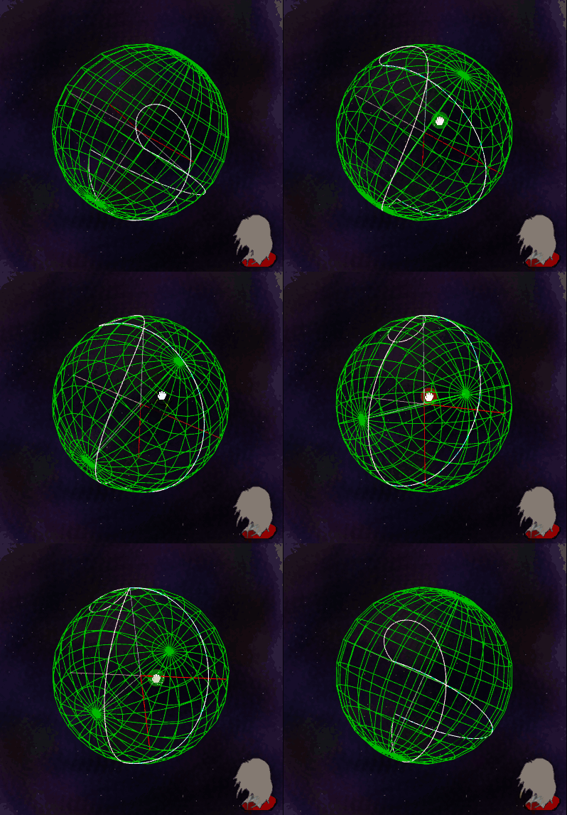
This web application is a tool for visually comparing and learning about quaternion (quaternion)
interpolation mechanisms used in 3D graphics and physics simulations.
The application draws the differences between quaternion interpolation paths,
which are abstract and difficult to understand, in real time based on the axis and angle set by the user.
-
Application Features
Users can freely set the rotation axis and angle of the start point (Src) and end point (Dest).
The application simultaneously calculates three interpolation paths to achieve the set rotation
and displays them on a sphere, color-coded. -
- Comparison of Interpolation Algorithms
The following three interpolation paths can be drawn and their differences can be visually compared.
- Comparison of Interpolation Algorithms
| Interpolation Method | Path Color | Characteristics | Mathematical Path |
|---|---|---|---|
| SLERP (Spherical Linear Interpolation) | Cyan (blue-green) | Travels the shortest distance (great arc) on a 4D unit sphere at a constant angular velocity. | Shortest arc |
| LERP (Linear Interpolation) | White (white) | Traces a straight line in 4D space and projects the result onto the sphere. The path is slightly concave toward the center of the sphere. | Straight line in 4D |
| LnQuat LERP (Logarithmic Space Linear Interpolation) | Pink | Converts quaternions to logarithmic space and performs linear interpolation (LSLERP) there. Ideally, it follows the same shortest path (great arc) as SLERP. | Logarithmic arc |
-
- Special Case Verification
This simulator can verify the following special behaviors, which are important
for deepening your understanding of quaternions.
- Special Case Verification
When rotation axes coincide: Even if the start and end axes are the same,
you can verify that interpolation according to the angle difference
is performed correctly. (LnQuat LERP has been debugged.)
Shortest path selection: If the SLERP/LERP is designed to intentionally
take a detour (a path that is not the shortest), you can verify
that only the LnQuat LERP shows the shortest path.
Visual difference: By changing the input parameters, you can verify
that the LERP line is slightly more concave toward the center of the sphere than the other two.
- Target audience
Students studying 3D game engines and graphics
Developers implementing quaternion-based motion and physics
Anyone who wants to visually understand the principles of quaternion interpolation
This section explains the fundamental concepts of camera and projection in 3D graphics, which are essential
for rendering 3D scenes onto a 2D screen. We'll focus on the relevant functionalities provided by the N6LMatrix and N6LVector libraries.
Simple Perspective Projection Test Demo & Explanation (External Link)
Note on Z-axis Sign Convention: In this section, the specific positive/negative direction of the Z-axis
in the projection formula is not intended to adhere to any particular standard convention.
The focus is on demonstrating the core mathematical concept of perspective projection using the provided frustum function.
This section outlines a basic demonstration of 3D wireframe rendering using only HTML Canvas
and custom mathematical calculations, without relying on external 3D libraries like Three.js or X3DOM.
It serves as a fundamental example of how perspective projection works from scratch.
Core Concepts and Formulas
The demonstration revolves around two primary transformations and their application:
-
Rotation Formula (Rodrigues' Rotation Formula Equivalent):
This rot function handles rotations of a 3D point p around an arbitrary axis a by an angle th.
This custom implementation directly reflects the mathematical principles of rotation.
function rot(a, th, p) {
  var c = Math.cos(th), s = Math.sin(th);
  return [
    (c + a[0] * a[0] * (1 - c)) * p[0] + (a[0] * a[1] * (1 - c) - a[2] * s) * p[1] + (a[0] * a[2] * (1 - c) + a[1] * s) * p[2],
    (a[1] * a[0] * (1 - c) + a[2] * s) * p[0] + (c + a[1] * a[1] * (1 - c)) * p[1] + (a[1] * a[2] * (1 - c) - a[0] * s) * p[2],
    (a[2] * a[0] * (1 - c) - a[1] * s) * p[0] + (a[2] * a[1] * (1 - c) + a[0] * s) * p[1] + (c + a[2] * a[2] * (1 - c)) * p[2]
  ];
}-
Near-Plane Perspective Projection Formula:
The frustum function implements a simple perspective projection onto a near plane.
A 3D point P = (Px, Py, Pz) is projected to a 2D point P' = (P'x, P'y) on the screen.
The formula used is:
P' = [ (n / Pz) * Px, (n / Pz) * Py ]
where n is the distance to the near plane.
function frustum(n, p) {
  return [(n / p[2]) * p[0], (n / p[2]) * p[1]];
}
Animation Loop Structure
The demonstration features an animation loop (GLoop) managed by a N6LTimerMan.
-
Entry Point and Main Loop Setup:
The enter3 function initializes the scene and sets up the main animation loop to run every 50 milliseconds.
function enter3() {
  init(); // Initializes 3D points and time
  TMan.add(); // Adds timer to manager
  TMan.timer[0].setalerm(function() { GLoop(0); }, 50); // Set main loop alarm
  return true;
}
Main Loop (GLoop):
Each frame, the GLoop function performs a series of transformations on the 3D points:
1.Combined Rotation: Points are successively rotated around the Z, Y, and X axes at different speeds.
2.Z-axis Translation: Points are translated along the Z-axis (e.g., rp[i][2] += 40) to adjust their distance from the camera.
3.Perspective Projection: Each transformed 3D point is then projected onto the 2D near plane using the frustum function.
4.Wireframe Drawing: The projected 2D points are connected to form the wireframe, which is then drawn on the HTML Canvas.
function GLoop(id) {
  // ... (time increment and variable declarations)
  // Rotation, Translation & Perspective Transformation
  for (i = 0; i < p.length; i++) rp[i] = rot([0, 0, 1], 1 * time, p[i]); // Z-axis rotation
  for (i = 0; i < rp.length; i++) rp[i] = rot([0, 1, 0], 2 * time, rp[i]); // Y-axis rotation
  for (i = 0; i < rp.length; i++) rp[i] = rot([1, 0, 0], 3 * time, rp[i]); // X-axis rotation
  for (i = 0; i < rp.length; i++) rp[i][2] += 40; // Z-axis translation
  for (i = 0; i < rp.length; i++) pp[i] = frustum(1, rp[i]); // Perspective projection
  // ... (Wireframe drawing on Canvas)
}The page also explains the fundamental principle behind converting a 2D screen coordinate back to a 3D world coordinate,
often referred to as "picking" or "ray casting."
Given the perspective projection formulas:
x = (n / Z) * X
y = (n / Z) * Y
The inverse transformations can be derived as:
X = (Z / n) * x
Y = (Z / n) * y
And from these, we can express Z:
Z = (n / x) * X
Z = (n / y) * Y
Combining these leads to the relationship between X and Y on the projected plane:
(n / x) * X = (n / y) * Y
X = (x / y) * Y or Y = (y / x) * X
The core idea is to:
1.Assume a 3D object's Z-coordinate (e.g., Z = -5 for an XY plane at that depth, with n = 1).
2.Calculate the corresponding X and Y coordinates: X = (Z / n) * x = 5x Y = (Z / n) * y = 5y
3.Essentially, the picking process involves starting from a known Z-coordinate
(e.g., the near plane Z=n) and iterating outwards (by increasing Z) until a 3D object is found
that satisfies the derived relationships between its 3D coordinates (X, Y, Z)
and the 2D screen coordinates (x, y). The first object encountered along this "ray" is the one "picked."
The View Matrix is crucial for positioning the viewer in a 3D scene. It transforms objects from the world coordinate system to the view space,
which is essentially the camera's perspective.
To make the camera "look at" a specific point in 3D space, N6LMatrix provides dedicated LookAtMat methods:
-
N6LMatrix.LookAtMat(eye, lookat, up):
This method creates a view matrix based on the camera's position (eye) in world space, the target point (lookat)
it's facing, and the camera's upward direction (up). Think of this as precisely aiming a real-world camera at a subject. -
N6LMatrix.LookAtMat2(rh):
This is an overloaded version of LookAtMat. It uses the N6LMatrix instance itself (presumably representing the camera's current pose)
as the eye position and rh as the lookat target to calculate the view matrix. This is useful for adjusting an existing camera's gaze.
Controlling camera motion primarily involves translation (movement) and rotation (orientation changes).
The N6LMatrix library offers powerful tools to achieve this:
-
N6LMatrix.MoveMat(outmat, outv, d, pyr, v, a, vmin, vmax):
This comprehensive method handles both camera movement and rotation in a single call.
outmat[0] and outv[0] are output parameters that return the matrix and velocity after the movement.
d: Represents the displacement vector for translation.
pyr: A 4-dimensional vector defining the camera's pitch, yaw, and roll.
v: The current velocity.
a: Acceleration.
vmin, vmax: Velocity limits (a value of 987654321.0 signifies no limit).
This method allows for integrated simulation of physics-based camera motion, including acceleration, deceleration, and velocity capping. -
N6LMatrix.TranslatedMat():
For simpler translational movements, this method generates a basic translation matrix. -
N6LMatrix.RotAxis() (and other rotation-related methods):
These methods generate rotation matrices, used for changing the camera's orientation. -
N6LMatrix.InverseMat(dt, sw):
This method calculates the inverse of a matrix, also providing its determinant. It's incredibly useful for deriving the view matrix
from a camera's world matrix, or for reverting complex transformations. The sw parameter offers flexibility
in choosing the inverse calculation algorithm.
By combining these functionalities, you can implement anything from interactive camera controls to automated camera paths in your 3D scenes.
After objects are transformed into view space, they are finally projected onto the 2D screen using a Projection Matrix.
There are two main types of projections: Perspective Projection and Orthographic Projection.
Perspective projection simulates how the human eye perceives depth: distant objects appear smaller, and closer objects appear larger.
It's essential for creating realistic 3D scenes with a sense of depth and scale.
-
N6LMatrix.FrustumMat(left, right, top, bottom, near, far): This method constructs the perspective projection matrix. Its parameters define the view frustum?the truncated pyramid
that represents the visible volume of the 3D world.
left, right, top, bottom: Coordinates of the left, right, top, and bottom clipping planes of the frustum.
near, far: Distances to the near and far clipping planes. These parameters collectively determine the field of view and aspect ratio,
defining which part of the 3D space will be projected onto the screen. -
N6LVector.FromLogAxis(base, range, x) / N6LVector.ToLogAxis(base, range, x): These methods facilitate conversions between logarithmic and normal axes. This is particularly useful for improving the precision
of the depth buffer in scenes containing both very near and very distant objects, mitigating Z-fighting issues. -
N6LVector.FrustumInfVec(base, range, v) / N6LVector.InvFrustumInfVec(base, range, v, z):
These methods are used for infinity perspective projection, a specialized form where the far clipping plane is conceptually at infinity,
often used for optimizing depth range.
Orthographic projection provides a view without perspective. Objects maintain their original size regardless of their distance from the camera,
making it ideal for CAD applications, 2D games, or technical drawings where consistent scale is crucial.
-
N6LMatrix.OrthoMat(left, right, top, bottom, near, far):
This method constructs the orthographic projection matrix. Its parameters define a rectangular bounding box that represents the visible volume.
left, right, top, bottom: Coordinates of the left, right, top, and bottom boundaries of the projection box.
near, far: Distances to the near and far clipping planes. Unlike perspective projection, all objects within this defined box will be projected
with their actual size, regardless of their depth.
HTML
<script src="https://nas6mixfoolv.github.io/NAS6LIB/javascripts/nas6lib/timer.js"></script>
JavaScript
// You do not usually need to wait for DOMContentLoaded to instantiate N6LTimerMan, but
// If there is processing that depends on other DOM elements, execute it in DOMContentLoaded.
var TMan = new N6LTimerMan(); // Assumes it is defined in NAS6LIB/javascripts/nas6lib/timer.js
var GLoopID = -1; //ID of Main Thread

//N6L initialization processing
function initializeN6L() {
  // Write the main processing for N6L initialization here.
  // For example, initializing calculations using N6LMatrix, obtaining Canvas and preparing drawing context.
  console.log("DOM is fully loaded. Initializing N6L...");

  GLoopID = TMan.add(); // Add a new timer to the timer manager
  GLoop(GLoopID); // Start the main thread by running it for the first time
}

//Main thread
function GLoop(id){
  // Write the main thread processing here.

  // Finally, reset the main thread to continue the thread, but if you do not reset it with an end condition, the thread will stop.
  TMan.timer[id].setalerm(function() { GLoop(id); }, 50); // Reset the main thread after 50 milliseconds.
}

// Add a DOMContentLoaded event listener
// It is standard to use window.document.addEventListener.
document.addEventListener('DOMContentLoaded', initializeN6L);

// Alternatively, you can use window.addEventListener('load', initializeN6L);
// DOMContentLoaded is faster and more suitable for DOM manipulation.
Example of code for calling the main thread 100 times and then automatically terminating it:
JavaScript
// You do not usually need to wait for DOMContentLoaded to instantiate N6LTimerMan, but
// If there is processing that depends on other DOM elements, execute it in DOMContentLoaded.
var TMan = new N6LTimerMan(); // Assumes it is defined in NAS6LIB/javascripts/nas6lib/timer.js
var GLoopID = -1; //ID of Main Thread

// add counter variable
var loopCount = 0;
const MAX_LOOP_COUNT = 100; // Define the number of ends

//N6L initialization processing
function initializeN6L() {
  // Write the main processing for N6L initialization here.
  // For example, initializing calculations using N6LMatrix, obtaining Canvas and preparing drawing context.
  console.log("DOM is fully loaded. Initializing N6L...");

  GLoopID = TMan.add(); // Add a new timer to the timer manager
  GLoop(GLoopID); // Start the main thread by running it for the first time
}

//Main thread
function GLoop(id){
  // Write the main thread processing here.
  console.log("Loop count: " + loopCount); // Display the current count (for debugging)

  // Increment the count
  loopCount++;

  // Check for exit condition
  if (loopCount <= MAX_LOOP_COUNT) {
    // Finally, reset the main thread to continue the thread, but if you don't reset it with an exit condition, the thread will stop.
    TMan.timer[id].setalerm(function() { GLoop(id); }, 50); // Reset the main thread after 50 milliseconds.
  } else {
    console.log("Main loop finished after " + MAX_LOOP_COUNT + " iterations.");
    //This is optional, but if you want strictness, please specify that it should be stopped.
    //TMan.timer[id].stop(); // Stop the timer and end the loop
  }
}

// Add a DOMContentLoaded event listener
// It is standard to use window.document.addEventListener.
document.addEventListener('DOMContentLoaded', initializeN6L);

// Alternatively, you can use window.addEventListener('load', initializeN6L);
// DOMContentLoaded is faster and more suitable for DOM manipulation.Back to Table of contents
Javascript multi-thread test using N6LTimerMan.htm DEMO
Javascript multi-thread test using N6LTimerMan.zip ZIP
./mttest.htm(Script part)
window.addEventListener("DOMContentLoaded", init);
var TMan = new N6LTimerMan(); //Timer manager
var pos = [ new N6LVector(4, true), new N6LVector(4, true), new N6LVector(4, true), new N6LVector(4, true)];
var th = [0, 0, 0, 0];
var dt = [50, 100, 150, 500];
var spd = 5.0;
var cnt = 0;
var div = 72;
var sph3;
var TManIDs = [];

function init() {
  const width = 500;
  const height = 250;

  const renderer = new THREE.WebGLRenderer({
    canvas: document.querySelector("#cnv0")
  });
  renderer.setPixelRatio(window.devicePixelRatio);
  renderer.setSize(width, height);
  const scene = new THREE.Scene();
  const camera = new THREE.PerspectiveCamera(
    45,
    width / height,
    1,
    10000
  );
  camera.position.set(0, 0, 20);

  // Create a sphere
  const sph0geometry = new THREE.SphereGeometry(1, 128, 128);
  // Set the color of the material
  const sph0material = new THREE.MeshBasicMaterial({ color: '#ff0000'});
  // Create a mesh
  const sph0 = new THREE.Mesh(sph0geometry, sph0material);
  sph0.position.set(0, 6, 0);
  pos[0] = new N6LVector([1, 0, 6, 0], true);
  // Create a sphere
  const sph1geometry = new THREE.SphereGeometry(1, 128, 128);
  // Set the color for the material
  const sph1material = new THREE.MeshBasicMaterial({ color: '#00ff00'});
  // Create a mesh
  const sph1 = new THREE.Mesh(sph1geometry, sph1material);
  sph1.position.set(0, 2, 0);
  pos[1] = new N6LVector([1, 0, 2, 0], true);
  // Create a sphere
  const sph2geometry = new THREE.SphereGeometry(1, 128, 128);
  // Set the color for the material
  const sph2material = new THREE.MeshBasicMaterial({ color: '#0000ff'});
  // Create a mesh
  const sph2 = new THREE.Mesh(sph2geometry, sph2material);
  sph2.position.set(0, -2, 0);
  pos[2] = new N6LVector([1, 0, -2, 0], true);
  // Create a sphere
  const sph3geometry = new THREE.SphereGeometry(1, 128, 128);
  // Set the color of the material
  const sph3material = new THREE.MeshBasicMaterial({ color: '#808080'});
  // Create a mesh
  sph3 = new THREE.Mesh(sph3geometry, sph3material);
  sph3.position.set(0, -6, 0);
  pos[3] = new N6LVector([1, 0, -6, 0], true);
  scene.add(sph0);
  scene.add(sph1);
  scene.add(sph2);
  scene.add(sph3);
  // Directional light source
  const light = new THREE.DirectionalLight(0xffffff);
  light.position.set(1, 1, 1);
  // Add to scene
  scene.add(light);

  // Create timer
  TManIDs = [TMan.add(), TMan.add(), TMan.add(), TMan.add(), TMan.add()];
  // First execution
  Loop0(TManIDs[0]);
  Loop1(TManIDs[1]);
  Loop2(TManIDs[2]);
  Loop3(TManIDs[3]);
  RDLoop(TManIDs[4]);

  function RDLoop(id) {

    // rendering
    renderer.render(scene, camera);
    TMan.timer[id].setalerm(function() { RDLoop(id); }, 50);
  }

  function Loop0(id) {

    th[id] += spd * Math.PI / 180.0;
    sph0.position.set(5 * Math.sin(th[id]) + pos[id].x[1], 6, 0);

    TMan.timer[id].setalerm(function() { Loop0(id); }, dt[id]);
  }

  function Loop1(id) {

    th[id] += spd * Math.PI / 180.0;
    sph1.position.set(5 * Math.sin(th[id]) + pos[id].x[1], 2, 0); TMan.timer[id].setalerm(function() { Loop1(id); }, dt[id]);
  }

  function Loop2(id) {

    th[id] += spd * Math.PI / 180.0;
    sph2.position.set(5 * Math.sin(th[id]) + pos[id].x[1], -2, 0);

    TMan.timer[id].setalerm(function() { Loop2(id); }, dt[id]);
  }

  function Loop3(id) {

    th[id] += spd * Math.PI / 180.0;

    var col1 = new N6LHsv(0, [255, 255, 0, 0]);
    var col2 = new N6LHsv(0, [255, 255, 0, 0]);
    var col = col1.HsvGrd(div, cnt, col2.ahsv, 1);
    var str = col.Str();
    cnt++;

    sph3.material.color.set(str);
    sph3.position.set(5 * Math.sin(th[id]) + pos[id].x[1], -6, 0);

    var c = (Math.cos(th[id]) + 1.0) / 2.0;
    dt[id] = 50 + c * 450; //Variable timer from 50 to 500[ms]

    TMan.timer[id].setalerm(function() { Loop3(id); }, dt[id]);
  }

}
var TMan = new N6LTimerMan(); //Timer manager
var pos = [ new N6LVector(4, true), new N6LVector(4, true), new N6LVector(4, true), new N6LVector(4, true)];
var th = [0, 0, 0, 0];
var dt = [50, 100, 150, 500];
var spd = 5.0;
...
var TManIDs = [];Key variables (TMan, pos, th, dt, spd)
Timer manager and ball position (pos), angle (th), speed (spd), multithread interval (dt)
Array for ID of each timer in the timer manager Declared
var cnt = 0;
var div = 72;
var sph3;
Used to change the color of the ball
Create a 3D scene in init()
//Create a timer
TManIDs = [TMan.add(), TMan.add(), TMan.add(), TMan.add(), TMan.add()];
Create five timers
//First execution
Loop0(TManIDs[0]);
Loop1(TManIDs[1]);
Loop2(TManIDs[2]);
Loop3(TManIDs[3]);
RDLoop(TManIDs[4]);
First execution of each
Previously, I was manually entering the ID magic number, but Gemini warned me to do it this way><
function RDLoop(id) {

  // Rendering
  renderer.render(scene, camera);
  TMan.timer[id].setalerm(function() { RDLoop(id); }, 50);
}
This is the rendering thread.
Loop0(),Loop1(),Loop2(),Loop3() are the threads for the movement of each ball.
Let's look at Loop0().
function Loop0(id) {

  th[id] += spd * Math.PI / 180.0;
  sph0.position.set(5 * Math.sin(th[id]) + pos[id].x[1], 6, 0);

  TMan.timer[id].setalerm(function() { Loop0(id); }, dt[id]);
}
th[id] += spd * Math.PI / 180.0;
th[id] is added by the angle spd degrees.
sph0.position.set(5 * Math.sin(th[id]) + pos[id].x[1], 6, 0);
The position calculated from the angle is applied to the sphere.
TMan.timer[id].setalerm(function() { Loop0(id); }, dt[id]);
Loop0(id) is called again at intervals of dt[id].
var dt = [50, 100, 150, 500];
is declared like this, so
Loop0 is called every 50ms, Loop1 every 100ms, and Loop2 every 150ms.
function Loop3(id) {

  th[id] += spd * Math.PI / 180.0;

  var col1 = new N6LHsv(0, [255, 255, 0, 0]);
  var col2 = new N6LHsv(0, [255, 255, 0, 0]);
  var col = col1.HsvGrd(div, cnt, col2.ahsv, 1);
  var str = col.Str();
  cnt++;

  sph3.material.color.set(str);
  sph3.position.set(5 * Math.sin(th[id]) + pos[id].x[1], -6, 0);

  var c = (Math.cos(th[id]) + 1.0) / 2.0;
  dt[id] = 50 + c * 450; // Variable timer from 50 to 500[ms]

  TMan.timer[id].setalerm(function() { Loop3(id); }, dt[id]);
}
Loop3
From col1(ARGB:FFFF0000,AHSV:100,0,100,100) to col2(ARGB:FFFF0000,AHSV:100,0,100,100)
Creates an HSV gradient around the RGB color wheel, divided into div(72) segments.
The color is applied with sph3.material.color.set(str);
var c = (Math.cos(th[id]) + 1.0) / 2.0;
dt[id] = 50 + c * 450; //50 to 500[ms] variable timer
The code is added, so it is a variable timer of 50 to 500[ms]
And so, multithreading can be achieved very easily using N6LTimerMan
Note that only one software timer is executed on the N6LTimerMan core
The timers managed by N6LTimerMan are distributed among the cores
so that resources are not strained as much as possible
Therefore, calling N6LTimer.add() many times does not have much effect. There is no problem.
Well, of course, timers with short intervals will put a load on the system.
The core operation of N6LTimerMan is to repeatedly run the core timer check thread
with one of the fastest software timers in N6LTimerMan.
measure the time, and when the time set by setalerm() for each timer has elapsed,
call the registered function for each timer.
That's all it does.
N6LTimerMan.changeinterval(INT); //Change timer check interval
You can set the core timer check interval with
Back to Table of contents
Back to NAS6LIB Repository [Links outside the wiki]