Get started
- First analysis example
- Analysis with cell segmentation
- Analysis with foci/transcription sites (cluster detection)
- Using several mono-channel images for segmentation
- Analysis without cytoplasm marker
Let's get started with a simple single molecule detection ! To launch small fish type in a terminal in your small fish environnement python -m small_fish_gui. This will launch small fish main menu, let's start with a simple detection by clicking on Add detection.
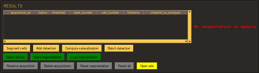
First step in any analysis will be to open your microscopy image in small fish, in the menu below click the Browse button and select your image file.
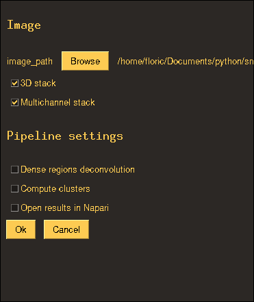
Then we have to help the software understands the axis it finds in the image, if your have several Z-stacks tick the 3D stack box and if you have several channels tick the Multichannel stack box. For this first analysis we will leave out the additional pipeline arguments. For this example I'm using a 3D, multichannel image.
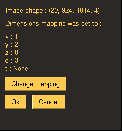
Small fish will then try to map the dimension axis in the right order, this usually works fine but in the case the shape presented on the top of the window (see below) click change mapping and fill in the boxes accordingly. Keep in mind that small fish is python based and the first axis is 0 not 1. When satistfied with axis mapping, proceed with Ok button.
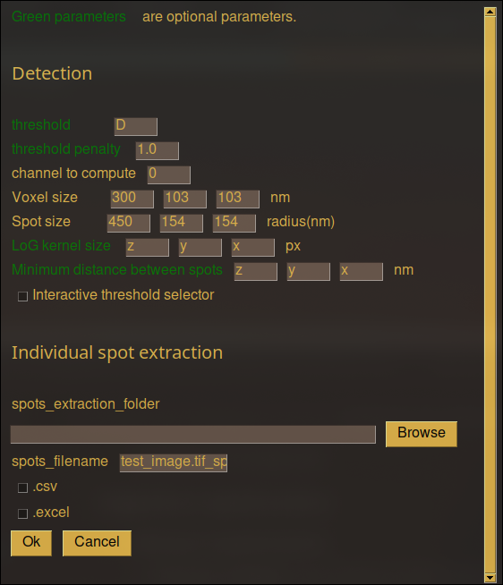
This will take you the detection parameter menu with a few prefilled parameters.
First you can take notice that parameters in green are optional. For spot detection 3 parameters are critical : voxel size, spot size, threshold. First the voxel size parameter is the size of a voxel (pixel) in nanometers, then spot size is the expected size of a single molecule in nanometers. For difraction limited spot I would recommend to set it between the voxel size and 1.5 x voxel size values. Finally, the threshold value can be optional in which case the software will try to infer a threshold, contrary to voxel size and spot size values which are parameters directly infered from the image caracteristic the threshold value is user dependent and correctly setting it will determine the quality of the measurements.
For this example let's leave out the threshold setting and go with the automatic setting instead tick the Interactive threshold selector.
The interactive threshold option will open a Napari interface before quantification in which you can try different threshold and spot sizes to fine tune your detection parameters. While fine-tuning your threshold remember that detection is performed in 3D and you might think is missed while it is detected on the layers above or below what you are looking, see here to learn how to visualize maximum projections or use the 3D mode.
In this interface you can also access the filtered image on which the threshold is applied. The filter applied on the image depends on both the voxel size and the spot size we previously set, for more insigth on the detection algorithm, check the detection section.
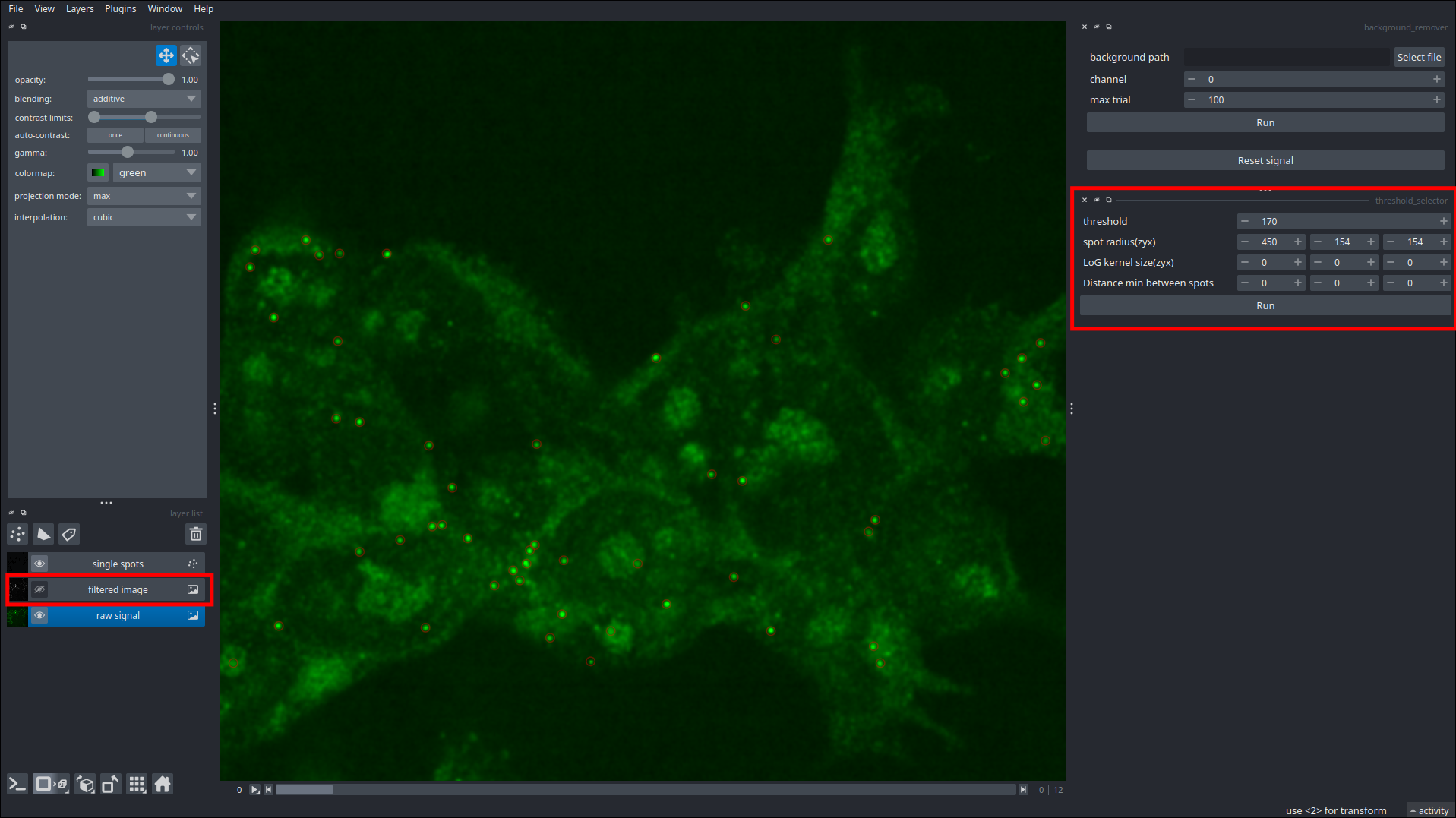
When satisfied with your threshold simply close napari. Small fish will then prompt you to valide the curret set of parameters or to restart if you whish to try other parameters.
After validating the parameters the quantification is performed and you will be taken back to main menu. To save you results simply click save results button and fill the prompt accordingly. Now let's have a look at the results :

In this file, because we analyzed only 1 image, we find one line of measurement with information like number of single molecules, single to noise ration, and all parameters that were used in this quantification. To view the full scope of the measurements available in Small Fish have a look at the Measurements section. Generally we are interested in cell to cell measurements which we can achieve by adding a step of segmentation to our analysis this will be the goal of our second example.
Let's proceed with an example of cell segmentation. There are two ways of achieving cell segmentation in Small Fish : with or without cytoplasm which means the software always expect to segment nuclei. Although if you don't have a nuclei marker, don't worry you can proceed anyway with your cytoplasm marker (or auto-fluorescence from cytoplasm) just consider that cytoplasm and nuclei are equivalent when setting parameters.
To beging we click on Segment cells in the main menu.
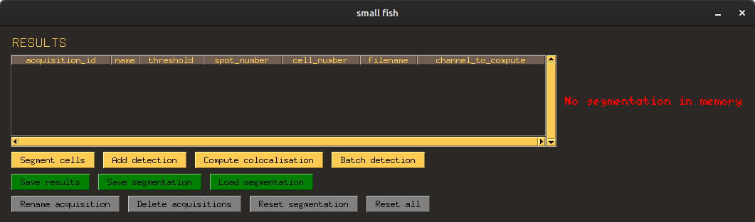
As for the first example, this will take you to the open image menu, when your image is correctly loaded and mapped you will proceed to the segmentation parameters prompt.
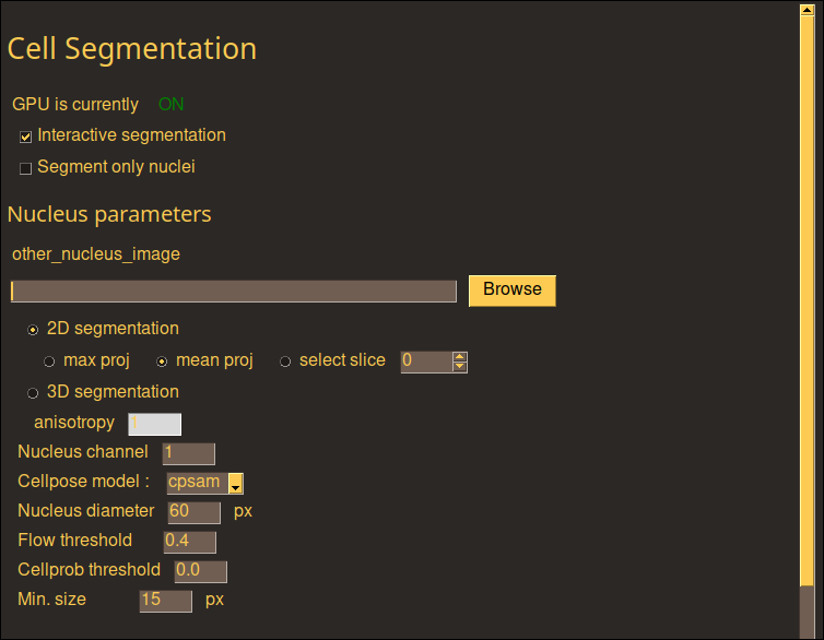
Segmentation now uses cellpose 4.0 and its new model cpsam which is very performant at the cost of heavy computational time which is why I warmly recommend setting up a GPU as indicated in the installation section. When the GPU is correctly set up you should read "GPU is currently ON" at the top of the window.
Cpsam model can be used for both nuclei and cytoplasm and usually yields good results even without going through a model retraining on you dataset. Note that contrary to the warning issued by cellpose in terminal at launch, the diameter parameter is NOT depreciated and highly impacts segmentation results.
For a first run you may try with all defaut parameters. Just make sure the channel for nuclei and cytoplasm are correctly set up and remember they start from 0 (ie. first channel is refered as 0).
Finally, we tick Interactive segmentation before launching the segmentation, this will show a Napari interface in which we can see and correct cellpose segmentation (see below).
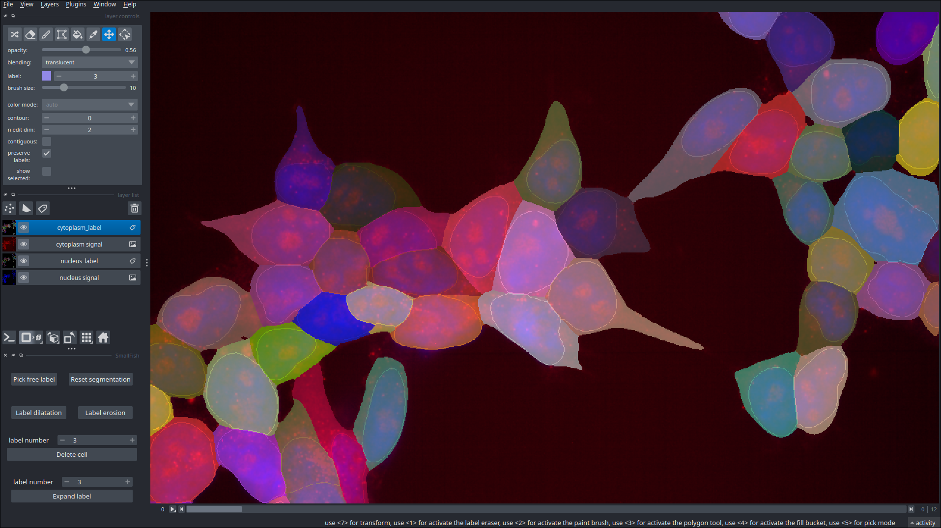
For more information on how to use segmentation tools in Napari see section User interface.
For more insight of how segmentation is handled see Segmentation section.
When satisfied with your segmentation simply close napari, then you can either restart segmentation with different parameters or validate you segmentation. This will take you back to main menu and you should see in gree segmentation in memory.
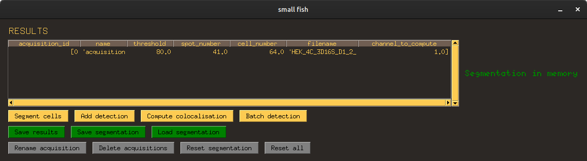
At this point you can click Add detection and proceed with spot detection as shown in example above. Afterwards you can save your results again with save results button and fill the prompt accordingly. This time an additional file named cell_results will be created and will contain all measurements for individual cells.
For our last example let us try to quantify some foci in cytoplasm, in this example I have ran the segmentation beforehand as shown in example above. I then proceed with Add detection and this time I also check the Dense regions deconvolution and the Compute clusters as well as the Open results in Napari options.
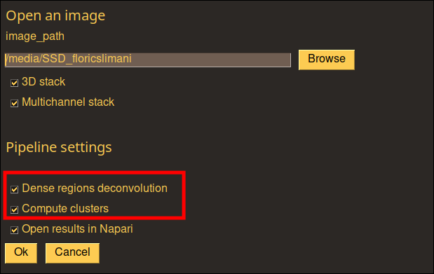
After correctly mapping your image you are once again prompted with detection parameters where you can find new parameters related to dense regions deconvolution and clustering. Firstly set up your voxel size and spot size parameters and tick the Interactive threshold selector. The new parameters are detailed in the detection section but for now let us try with default parameters as we will be able to fine tune them in the napari interface.
Again we can play with the spot size and threshold parameters to achieve spot detection, keep in mind that those parameters should be set to detect individual spots and not clusters.
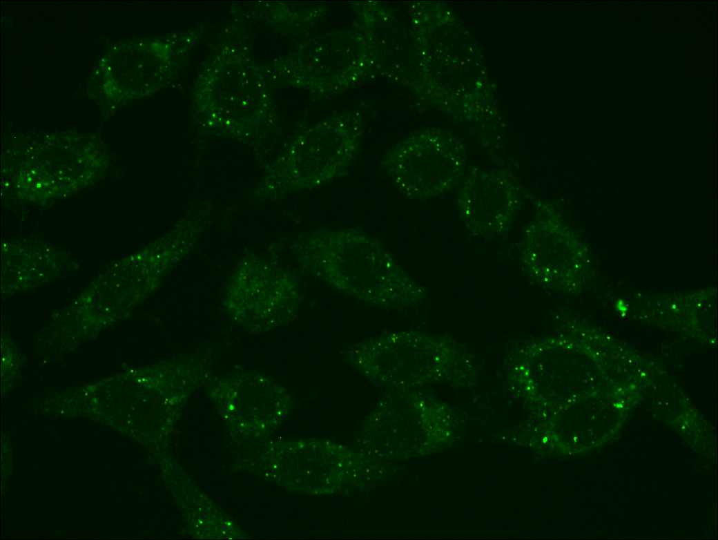
Now let us consider the clustering part, many fish experiments aim at quantifying foci, transcription site, number of nascent rna at transcription site and so on. In Small fish transcription sites and foci are considered as clusters. To detect them the software will try to find region where there is a dense localization of individual spots, however due to the diffraction limit what appears as a very bright spot can actually be the agglomeration of many individual spot in such a way that the microscope could not resolve it. This is where dense regions deconvolution comes in as it aims at modelizing the number of individual spot composing the bright signal, again to learn more insight about this process and associated parameters check the detection section.
For this example let us proceed again with default parameters by clicking the run button under the dense regions deconvolution parameters.
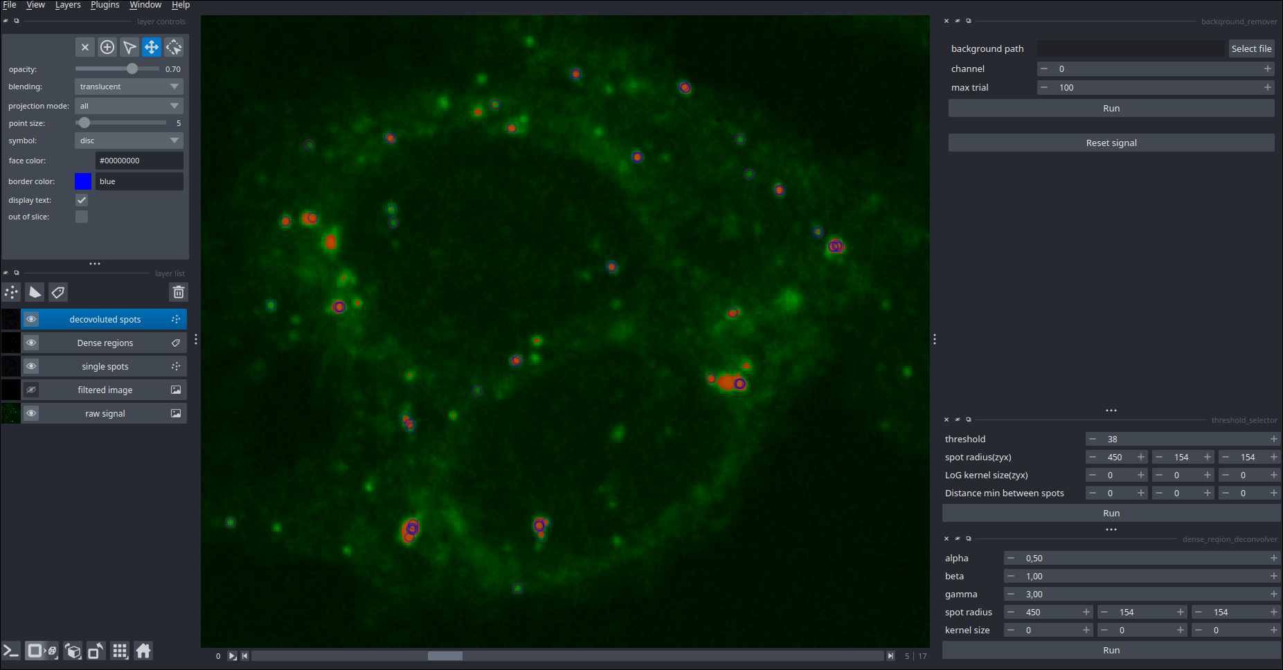
After computing two new layers are added to the viewer : Dense regions and deconvoluted spots.
Dense regions is will show in red the pixels that are considered as part of the regions where we should try to add spots, it is critical that it covers what you aim at quantifying as foci or transcription site but can cover other region as well. The deconvoluted spots layers (in blue) contains all the spots detected plus newly added by the deconvolution those spots will be the one considered when trying to find clusters. When satisfied close the napari viewer to proceed, after a computing time a new napari window will open (due to our ticking Open results in Napari).
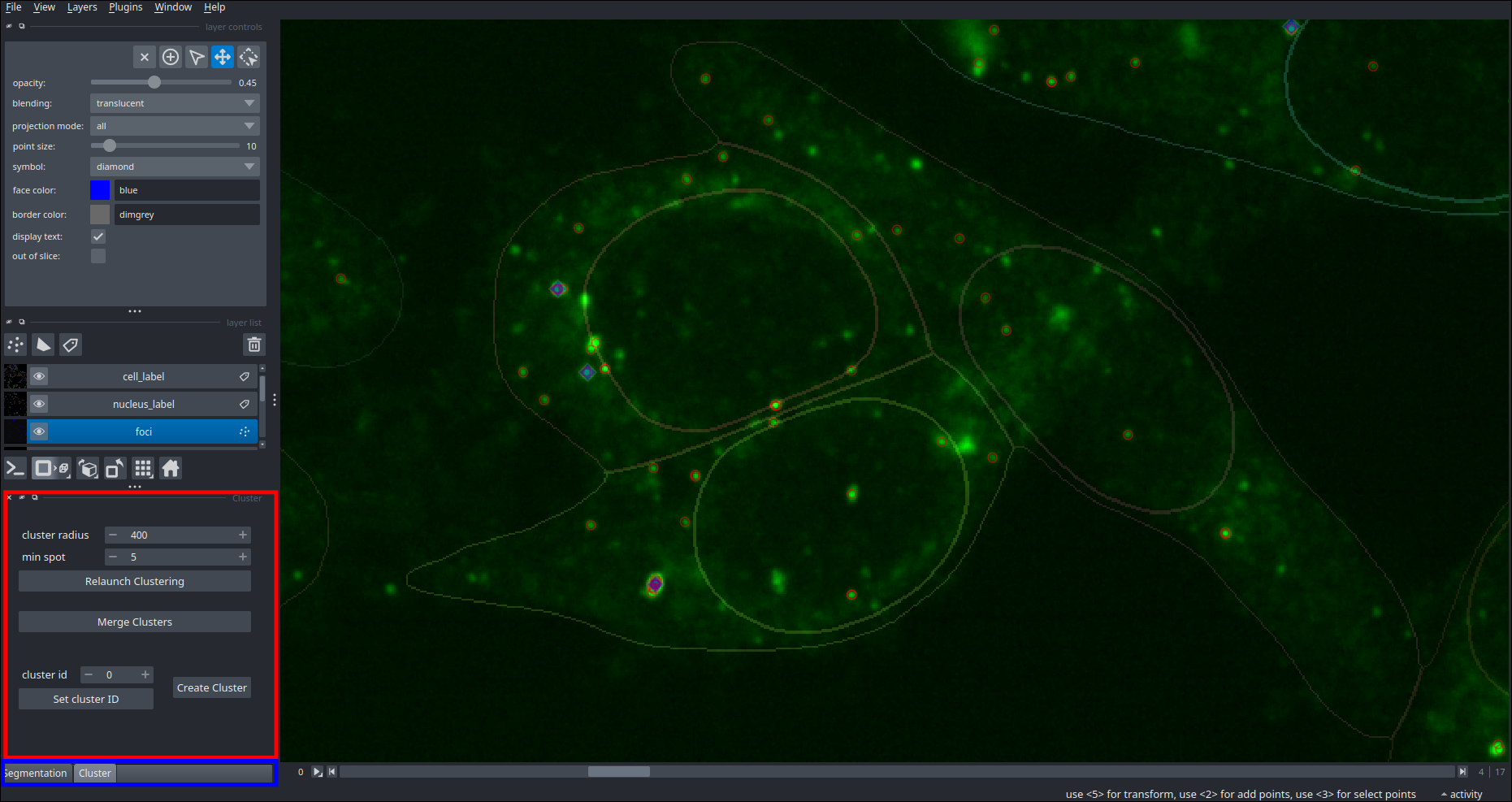
This interface is your last opportunity to impact the quantification, it is aimed both to interact with the clustering processing and to visualize exactly what the software will quantify. Here you will find you all the channel present in your cells (to take pretty pictures), nuclei and cytoplasm labels (if any), the detected spots (in red) and the clusters as blue diamonds. You can try to play with clustering parameters but again more details can be found in the detection and interface sections.
To launch quantification close the napari window you will be returned to main menu upon completion. After saving results a few more columns are added to the measurements note that extracting data at individual spot level is also possible enabling further quantification on spots and clustering, see the spot extraction procedure.
Still uncomfortable with how the interface works ? Check the user interface section.