MaAsLin2
MaAsLin 2 is the next generation of MaAsLin (Microbiome Multivariable Association with Linear Models).
MaAsLin 2 is a comprehensive R package for efficiently determining multivariable association between phenotypes, environments, exposures, covariates and microbial meta-omics features. MaAsLin 2 relies on general linear models to accommodate most modern epidemiological study designs, including cross-sectional and longitudinal, along with a variety of data exploration, normalization, and transformation methods.
If you use the MaAsLin 2 software, please cite our manuscript:
Mallick H, Rahnavard A, McIver LJ, Ma S, Zhang Y, Nguyen LH, Tickle TL, Weingart G, Ren B, Schwager EH, Chatterjee S, Thompson KN, Wilkinson JE, Subramanian A, Lu Y, Waldron L, Paulson JN, Franzosa EA, Bravo HC, Huttenhower C (2021). Multivariable Association Discovery in Population-scale Meta-omics Studies. PLoS Computational Biology, 17(11):e1009442.
If you have questions, please direct it to :
MaAsLin 2 Forum
Google Groups (Read only)
- 1. Installing R
- 2. Installing MaAsLin 2
- 3. Microbiome Association Detection with MaAsLin 2
- 4. Advanced Topics
- 5. Command Line Interface
R is a programming language specializing in statistical computing and graphics. You can use R just the same as any other programming languages, but it is most useful for statistical analyses, with well-established packages for common tasks such as linear modeling, 'omic data analysis, machine learning, and visualization. We have created a short introduction tutorial here, but we note there are many other more comprehensive tutorials out there to learn R.
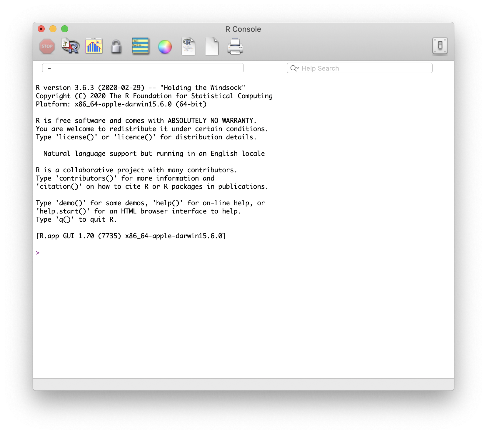
You can download and install the free R software environment here. Note that you should download the latest release - this will ensure the R version you have is compatible with MaAsLin 2. Once you've finished the installation, locate the R software and launch it - you should have a window that looks like this:
RStudio is a freely available IDE (integrated development environment) for R. It is a "wrapper" around R with some additional functionalities that makes programming in R a bit easier. Feel free to download RStudio and explore its interface - but it is not required for this tutorial.
If you already have R installed, then it is possible that the R version you have
does not support MaAsLin 2. The easiest way to check this is to launch R/RStudio,
and in the console ("Console" pane in RStudio), type in the following command
(without the > symbol):
> sessionInfo()The first line of output message should indicate your current R version. For example:
> sessionInfo()
R version 3.6.3 (2020-02-29)
For MaAsLin 2 to install, you will need R >= 3.6.0. If your version is older than
that, please refer to section
Installing R for the first time to download
the latest R. Note that
RStudio users will need to have RStudio "switch" to this later version once it
is installed. This should happen automatically for Windows and Mac OS users when
you relaunch RStudio. For Linux users you might need to bind the correct R
executable. For more information refer to here. Either way, once you have the correct version installed, launch
the software and use sessionInfo() to make sure that you indeed have R >= 3.6.0.
Once you have the correct R version, you can install MaAsLin 2 with Bioconductor:
if(!requireNamespace("BiocManager", quietly = TRUE))
    install.packages("BiocManager")
BiocManager::install("Maaslin2")You might encounter an error message that states:
Warning message:
package ‘Maaslin2’ is not available (for R version x.x.x)
This can be due to one of two reasons:
-
Your R version is too old. Check this with
sessionInfo()- if it is older than 3.6, download the most updated version per instructions above. -
You have an older version of Bioconductor. MaAsLin2 requires Bioconductor >= 3.10. You can check your Bioconductor version with
BiocManager::version(). If the returned version is anything older than 3.10, you can update with
BiocManager::install(version = "3.10")And then
BiocManager::install("Maaslin2")This is a place-holder right now.
Set up
Launch a fresh R session and in the R script window:
getwd()
setwd("~/Desktop")
dir.create("R_Maaslin_tutorial") # Create a new directory
setwd("R_Maaslin_tutorial") # Change the current working directory
getwd() #check if directory has been successfully changed

#Load MaAsLin 2 package into the R environment
library(Maaslin2)
?Maaslin2
MaAsLin 2 requires two input files, one for taxonomic or functional feature abundances, and one for sample metadata.
- Data (or features) file
- This file is tab-delimited.
- Formatted with features as columns and samples as rows.
- The transpose of this format is also okay.
- Possible features in this file include microbes, genes, pathways, etc.
- Metadata file
- This file is tab-delimited.
- Formatted with features as columns and samples as rows.
- The transpose of this format is also okay.
The data file can contain samples not included in the metadata file (along with the reverse case). For both cases, those samples not included in both files will be removed from the analysis. Also the samples do not need to be in the same order in the two files.
Example input files can be found in the inst/extdata folder
of the MaAsLin 2 source. The files provided were generated from
the HMP2 data which can be downloaded from https://ibdmdb.org/ .
input_data = system.file("extdata", "HMP2_taxonomy.tsv", package="Maaslin2") # The abundance table file
input_data

input_metadata = system.file("extdata", "HMP2_metadata.tsv", package="Maaslin2") # The metadata table file
input_metadata

#get the pathway (functional) data - place holder
download.file("https://raw.githubusercontent.com/biobakery/biobakery_workflows/master/examples/tutorial/stats_vis/input/pathabundance_relab.tsv", "./pathabundance_relab.tsv")
HMP2_taxonomy.tsv: is a tab-demilited file with species as columns and
samples as rows. It is a subset of the taxonomy file so it just includes the
species abundances for all samples.
HMP2_metadata.tsv: is a tab-delimited file with samples as rows and metadata
as columns. It is a subset of the metadata file so that it just includes some of
the fields.
pathabundance_relab.tsv: is a tab-delimited file with samples as columns and pathway level features
as rows. It is a subset of the pathway file so it just includes the
species abundances for all samples.
Saving inputs as data frames
df_input_data = read.table(file             = input_data,
                           header           = TRUE,
                           sep              = "\t",
                           row.names        = 1,
                           stringsAsFactors = FALSE)
df_input_data[1:5, 1:5]

df_input_metadata = read.table(file             = input_metadata,
                               header           = TRUE,
                               sep              = "\t",
                               row.names        = 1,
                               stringsAsFactors = FALSE)
df_input_metadata[1:5, ]

df_input_path = read.csv("./pathabundance_relab.tsv",
                         sep              = "\t",
                         stringsAsFactors = FALSE,
                         row.names        = 1)
df_input_path[1:5, 1:5]Several different types of statistical models can be used for association testing in MaAsLin (e.g. simple linear, zero-inflated, count-based, etc.). We have evaluated their pros and cons in the associated manuscript, and while the default is generally appropriate for most analyses, a user might want to select a different model under some circumstances. This is true for many different microbial community data types (taxonomy or functional profiles), environments (human or otherwise), and measurements (counts or relative proportions), as long as alternative models are used with appropriately modified normalization/transformation schemes.
- For models, if your inputs are counts, then you can use
NEGBINandZINB, whereas, for non-count (e.g. percentage, CPM, or relative abundance) input, you can useLMandCPLM. - Among the normalization approaches implemented in MaAsLin 2,
TMMandCSSonly work on counts, and they also return normalized counts, unlikeTSSandCLR. Therefore, if your inputs are counts, you can use the above two normalizations (i.e.,TMM,CSS, orNONE(in case the data is already normalized)) without a further transformation (i.e. transform =NONE). - Among the non-count models,
CPLMrequires the data to be positive. Therefore, any transformation that produces negative values will typically NOT work forCPLM. - All the non-LM models use an intrinsic log link transformation due to their close connection to GLMs and they are recommended to be run with
transform = NONE. - Apart from that,
LMis the only model that works on both positive and negative values (following normalization/transformation), and (as per our manuscript), it is generally much more robust to parameter changes (which are typically limited for non-LM models). Regarding whether to useLM,CPLM, or other models, intuitively,CPLMor a zero-inflated alternative should perform better in the presence of zeroes, but based on our benchmarking, we do not have evidence thatCPLMis significantly better thanLMin practice.
| Model (-m ANALYSIS_METHOD) | Data type | Normalization (-n NORMALIZATION) | Transformation (-t TRANSFORM) |
|---|---|---|---|
| LM | count and non-count |
TSS,CLR, NONE
|
LOG, LOGIT, AST,NONE
|
| CPLM | count and non-count |
TSS, TMM, CSS, NONE
|
NONE |
| NEGBIN | count |
TMM, CSS, NONE
|
NONE |
| ZINB | count |
TMM, CSS, NONE
|
NONE |
NOTE: generally you will also need to consider what thresholds you have used to filter the data (i.e. the prevalence and abundance threshold) to reduce outliers and false positives. See section 4.3.1 Prevalence and abundance filtering in MaAsLin 2 for some more details on this.
The following command runs MaAsLin 2 on the HMP2 data, running a multivariable
regression model to test for the association between microbial species abundance
versus IBD diagnosis and dysbiosis scores
(fixed_effects = c("diagnosis", "dysbiosis")). For any categorical variable with more than 2 levels, you will also have to specify which variable should be the reference level by using (reference = c("diagnosis,nonIBD")). NOTE: adding a space between the variable and level might result in the wrong reference level being used. Output are generated in a folder called demo_output under the current working directory (output = "demo_output"). In this case, the example input data has been pre-normalized and pre-filtered, so we turn off the default normalization and prevalence filtering as well.
fit_data = Maaslin2(input_data     = input_data,
                    input_metadata = input_metadata,
                    min_prevalence = 0,
                    normalization  = "NONE",
                    output         = "demo_output",
                    fixed_effects  = c("diagnosis", "dysbiosis"),
reference = c("diagnosis,nonIBD"))If you are familiar with the data frame class in R, you can also provide data
frames for input_data and input_metadata for MaAsLin 2, instead of
file names. One potential benefit of this approach is that it allows you to
easily manipulate these input data within the R environment.
fit_data2 = Maaslin2(input_data     = df_input_data,
                     input_metadata = df_input_metadata,
                     min_prevalence = 0,
                     normalization  = "NONE",
                     output         = "demo_output2",
                     fixed_effects  = c("diagnosis", "dysbiosis"),
reference = c("diagnosis,nonIBD"))- Question: how would I run the same analysis, but only on CD and nonIBD
subjects?
- Hint: try
?dplyr::filter()
- Hint: try
Perhaps the most important output from MaAsLin 2 is the list of significant
associations. These are provided in significant_results.tsv:
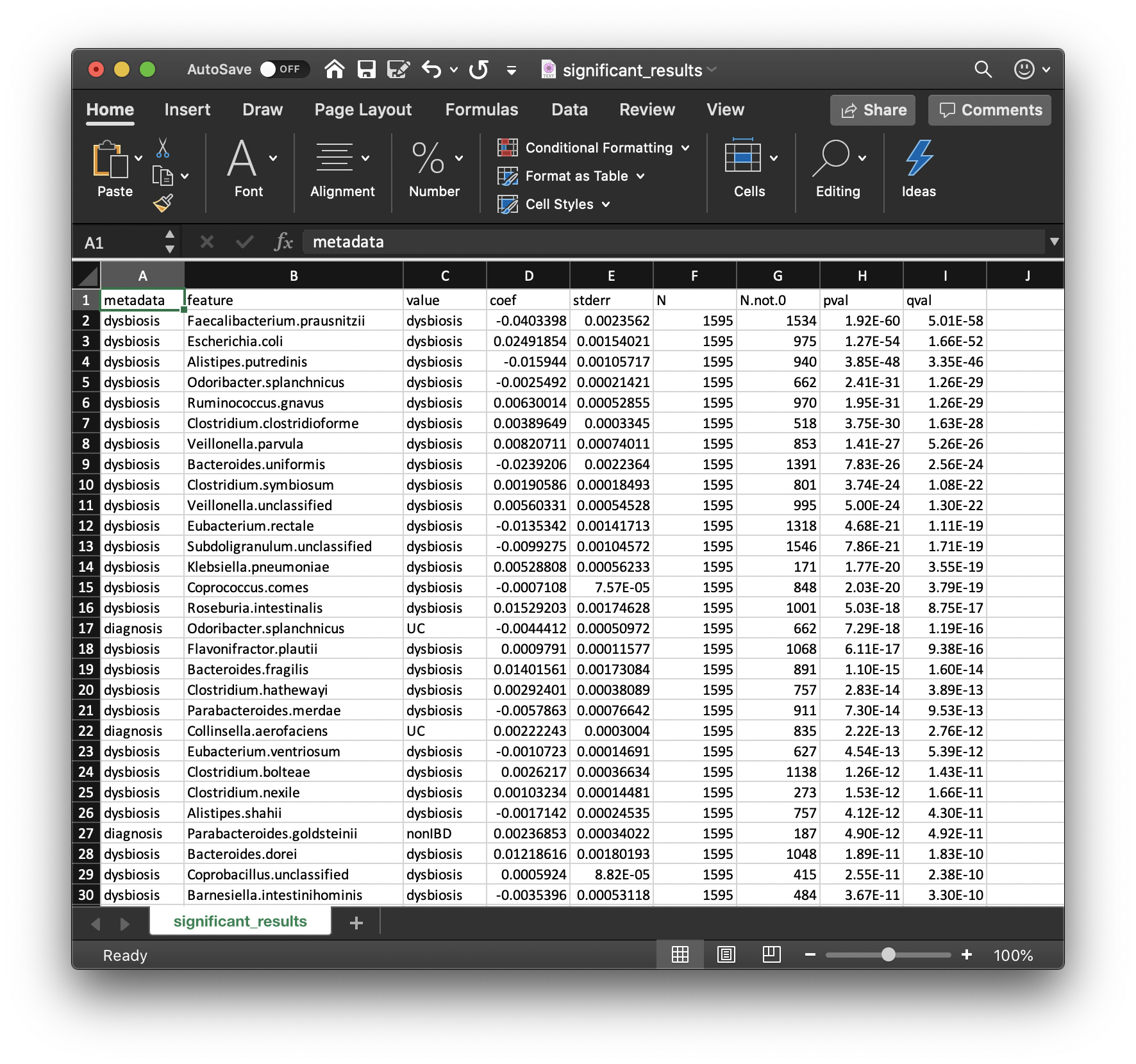
These are the full list of associations that pass MaAsLin 2's significance threshold, ordered by increasing q-values. Columns are:
-
metadata: the variable name being associated with a microbial feature. -
feature: the microbial feature (taxon, gene, pathway, etc.). -
value: for categorical features, the specific feature level for which the coefficient and significance of association is being reported. -
coef: the model coefficient value (effect size).- Coefficients for categorical variables indicate the contrast between the
category specified in
valueversus the reference category.
- Coefficients for categorical variables indicate the contrast between the
category specified in
-
stderr: the standard error from the model. -
N: the total number of samples used in the model for this association (since e.g. missing values can be excluded). -
N.not.0: the total of number of these samples in which the feature is non-zero. -
pval: the nominal significance of this association. -
qval: the corrected significance is computed withp.adjustwith the correction method (BH, etc.). -
Question: how would you interpret the first row of this table?
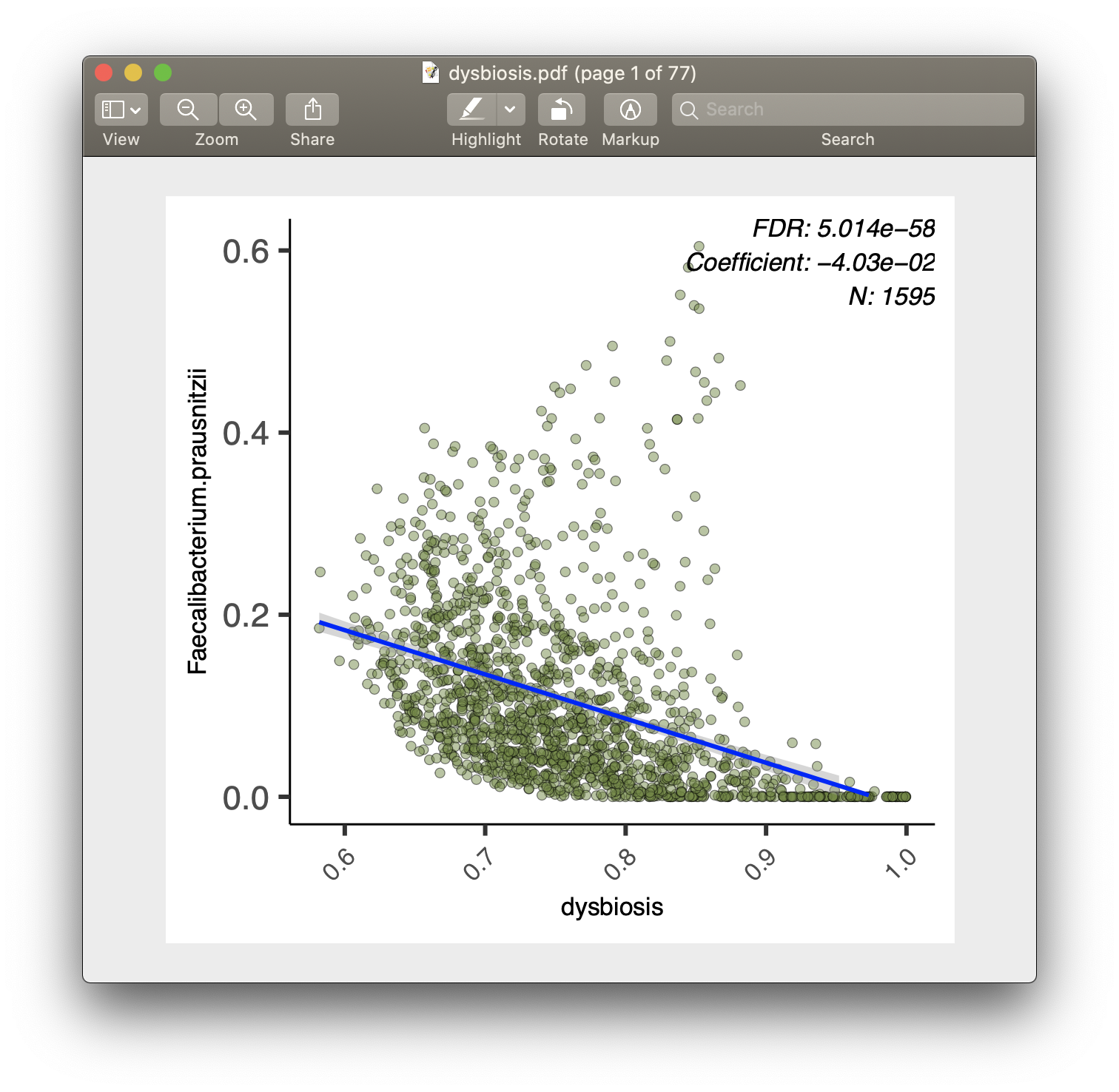
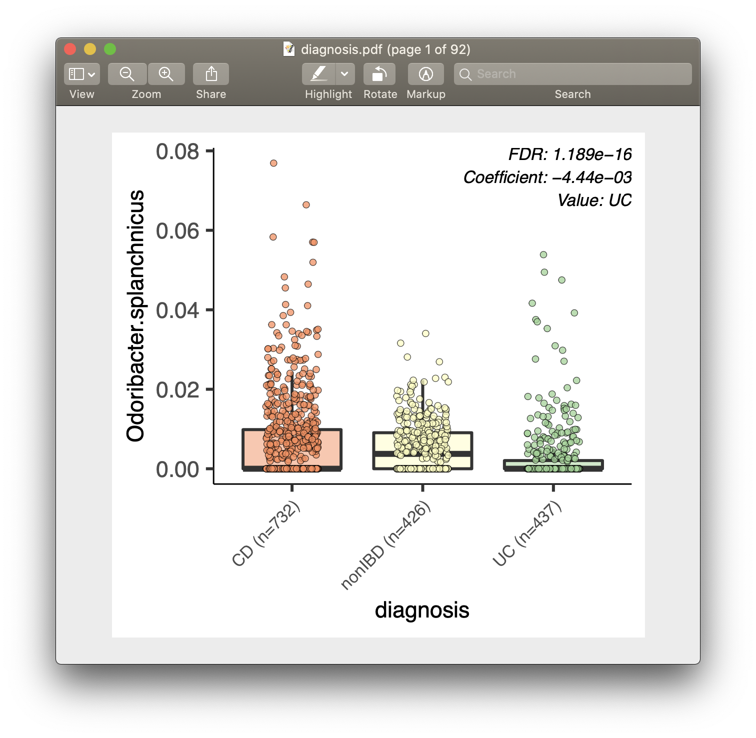
For each of the significant associations in significant_results.tsv, MaAsLin 2
also generates visualizations for inspection (boxplots for categorical variables,
scatter plots for continuous). These are named as "metadata_name.pdf". For
example, from our analysis run, we have the visualization files dysbiosis.pdf
and diagnosis.pdf:
MaAsLin 2 generates two types of output files: data and visualization.
- Data output files
-
significant_results.tsv- As introduced above.
-
all_results.tsv- Same format as
significant_results.tsv, but include all association results (instead of just the significant ones). - You can also access this table within R using
fit_data$results.
- Same format as
-
residuals.rds- This file contains a data frame with residuals for each feature.
-
maaslin2.log- This file contains all log information for the run.
- It includes all settings, warnings, errors, and steps run.
-
- Visualization output files
-
heatmap.pdf- This file contains a heatmap of the significant associations.
-
[a-z/0-9]+.pdf- A plot is generated for each significant association.
- Scatter plots are used for continuous metadata.
- Box plots are for categorical data.
- Data points plotted are after normalization, filtering, and transform.
-
If your functional tables have been produced by HUMAnN and been normalized with the humann_renorm_table script, then you don’t need to perform any additional normalization – the effects of sequencing depth will have already been removed (which is what we will be using in this tutorial). We tend to work with CPM units because we find them to be more convenient, but they are numerically equivalent to relative abundances for modeling purposes (CPM = RA * 1e6).
Otherwise - you will want to use the same thoughts above about model/normalization/transformation as above.
Some other quick tips for using MaAsLin 2 on functional profiles:
- To reduce the number of features, you typically want to run either the unstratified functional features (or a filtered subset of the stratified features)
- You may also want to remove functional features that are highly correlated to one specific taxon (i.e. likely contributed by that microbe), since these can be better-explained by taxonomic changes.
#This can also be done with with the HUMAnN 3 untiliy `humann_split_stratified_table`
unstrat_pathways <-function(dat_path){
  temp = dat_path[!grepl("\\|",rownames(dat_path)),]
  return(temp)
}

df_input_path = unstrat_pathways(df_input_path)
Run the same model as above on the MetaCyc pathway table generated from the bioBakery workflows.
fit_func = Maaslin2(input_data     = df_input_path,
                    input_metadata = df_input_metadata,
                    output         = "demo_functional",
                    fixed_effects  = c("diagnosis", "dysbiosis"),
                    reference      = c("diagnosis,nonIBD"),
                    min_abundance  = 0.0001,
                    min_prevalence = 0.1)
Note: Here we have the samples in the columns and the features in the rows and MaAsLin 2 correctly identified this and was able to match the samples.
We have also recently published on using MaAsLin 2 to analyze differential features in metatranscriptomic data (MTX), for further information on that please see our recent publication.
Some helpful tips and tricks (HUMAnN related)
Q: Does the output of the functional run make sense? What are some of the important features to investigate further?
Many statistical analysis are interested in testing for interaction
between certain variables. Unfortunately, MaAsLin 2 does not yet provide a direct
interface for this. Instead, the user needs to create artificial interaction
columns as additional fixed_effects terms. Using the above fit as an example,
to test for the interaction between diagnosis and dysbiosis, I
can create two additional columns: CD_dysbiosis and UC_dysbiosis (since the
reference for diagnosis is nonIBD):
df_input_metadata$CD_dysbiosis = (df_input_metadata$diagnosis == "CD") *
                                 df_input_metadata$dysbiosis
df_input_metadata$UC_dysbiosis = (df_input_metadata$diagnosis == "UC") *
                                 df_input_metadata$dysbiosis

fit_data_ixn = Maaslin2(input_data     = df_input_data,
                        input_metadata = df_input_metadata,
                        min_prevalence = 0,
                        normalization  = "NONE",
                        output         = "demo_output_interaction",
                        fixed_effects  = c("diagnosis", "dysbiosis", "CD_dysbiosis", "UC_dysbiosis"),
reference = c("diagnosis,nonIBD"))Certain studies have a natural "grouping" of sample observations, such
as by subject in longitudinal designs or by family in family designs. It is
important for statistic analysis to address the non-independence between samples
belonging to the same group MaAsLin 2 provides a simple interface for this
through the parameter random_effects, where the user can specify the grouping
variable to run a mixed effect model instead. For
example, we note that HMP2 is a longitudinal design where the same subject
(column subject) can have multiple samples. We thus ask MaAsLin 2 to use
subject as its random effect grouping variable:
fit_data_random = Maaslin2(input_data     = df_input_data,
                           input_metadata = df_input_metadata,
                           min_prevalence = 0,
                           normalization  = "NONE",
                           output         = "demo_output_random",
                           fixed_effects  = c("diagnosis", "dysbiosis"),
                           random_effects = c("subject"),
                           reference      = c("diagnosis,nonIBD"))
If you are interested in testing the effect of time in a longitudinal study,
then the time point variable should be included in fixed_effects during your
MaAsLin 2 call.
- Question: intuitively, can you think of a reason why it is important to
address non-independence between samples?
- Hint: imagine the simple scenario where you have two subject, one case and one control, each has two samples.
- What is the effective sample size, when samples of the same subject are highly independent, versus when they are highly correlated?
MaAsLin 2 provide many parameter options for different data pre-processing (normalization, filtering, transfomation) and other tasks. The full list of these options are:
-
min_abundance- The minimum abundance for each feature [ Default:
0]
- The minimum abundance for each feature [ Default:
-
min_prevalence- The minimum percent of samples for which a feature is detected at minimum
abundance [ Default:
0.1]
- The minimum percent of samples for which a feature is detected at minimum
abundance [ Default:
-
max_significance- The q-value threshold for significance [ Default:
0.25]
- The q-value threshold for significance [ Default:
-
normalization- The normalization method to apply [ Default:
"TSS"] [ Choices:"TSS","CLR","CSS","NONE","TMM"]
- The normalization method to apply [ Default:
-
transform- The transform to apply [ Default:
"LOG"] [ Choices:"LOG","LOGIT","AST","NONE"]
- The transform to apply [ Default:
-
analysis_method- The analysis method to apply [ Default:
"LM"] [ Choices:"LM","CPLM","ZICP","NEGBIN","ZINB"]
- The analysis method to apply [ Default:
-
correction- The correction method for computing the
q-value [ Default:
"BH"]
- The correction method for computing the
q-value [ Default:
-
standardize- Apply z-score so continuous metadata are
on the same scale [ Default:
TRUE]
- Apply z-score so continuous metadata are
on the same scale [ Default:
-
plot_heatmap- Generate a heatmap for the significant
associations [ Default:
TRUE]
- Generate a heatmap for the significant
associations [ Default:
-
heatmap_first_n- In heatmap, plot top N features with significant
associations [ Default:
50]
- In heatmap, plot top N features with significant
associations [ Default:
-
plot_scatter- Generate scatter plots for the significant
associations [ Default:
TRUE]
- Generate scatter plots for the significant
associations [ Default:
-
cores- The number of R processes to run in parallel
[ Default:
1]
- The number of R processes to run in parallel
[ Default:
-
reference- The factor to use as a reference for a variable with more than two levels provided as a string of 'variable,reference' semi-colon delimited for multiple variables.
Typically, it only makes sense to test for feature-metadata associations if a feature is non-zero "enough" of the time. "Enough" can vary between studies, but a 10-50% minimum prevalence threshold is not unusual (and up to 70-90% can be reasonable). Since we're already using a small, selected subset of demo data, we'll use min_prevalence = 0.1 to test only features with at least 10% non-zero values. Note: this is the default parameter setting in MaAsLin 2.
Similarly, it's often desirable to test only features that reach a minimum abundance threshold in at least this many samples. By default, MaAsLin 2 will consider any non-zero value to be reliable, and if you've already done sufficient QC in your dataset, this is appropriate. However, if you'd like to filter more or be conservative, you can set a minimum abundance threshold like min_abundance = 0.0001 to test only features reaching at least this (relative) abundance.
Putting these arguments together, we can run MaAsLin 2 (and it'll go even faster!) using both:
fit_data_filter = Maaslin2(input_data     = df_input_data,
                           input_metadata = df_input_metadata,
                           normalization  = "NONE",
                           output         = "demo_output_filter",
                           fixed_effects  = c("diagnosis", "dysbiosis"),
                           reference      = c("diagnosis,nonIBD"),
                           random_effects = c("subject"),
                           min_prevalence = 0.1,
min_abundance = 0.0001)MaAsLin 2 can also be run with a command line interface. For example, the demo analysis can be performed with:
Maaslin2.R --transform=AST --fixed_effects="diagnosis,dysbiosis" /usr/local/lib/R/site-library/Maaslin2/extdata/HMP2_taxonomy.tsv /usr/local/lib/R/site-library/Maaslin2/extdata/HMP2_metadata.tsv demo_output --reference="diagnosis,nonIBD"
- Make sure to provide the full path to the MaAsLin 2 executable (ie ./R/Maaslin2.R).
- In the demo command:
-
HMP2_taxonomy.tsvis the path to your data (or features) file -
HMP2_metadata.tsvis the path to your metadata file -
demo_outputis the path to the folder to write the output
-
Full help documentation:
$ Maaslin2.R --help
Usage: ./R/Maaslin2.R [options] <data.tsv> <metadata.tsv> <output_folder>

Options:
    -h, --help
        Show this help message and exit

    -a MIN_ABUNDANCE, --min_abundance=MIN_ABUNDANCE
        The minimum abundance for each feature [ Default: 0 ]

    -p MIN_PREVALENCE, --min_prevalence=MIN_PREVALENCE
        The minimum percent of samples for which a feature
        is detected at minimum abundance [ Default: 0.1 ]

    -s MAX_SIGNIFICANCE, --max_significance=MAX_SIGNIFICANCE
        The q-value threshold for significance [ Default: 0.25 ]

    -n NORMALIZATION, --normalization=NORMALIZATION
        The normalization method to apply [ Default: TSS ]
        [ Choices: TSS, CLR, CSS, NONE, TMM ]

    -t TRANSFORM, --transform=TRANSFORM
        The transform to apply [ Default: LOG ]
        [ Choices: LOG, LOGIT, AST, NONE ]

    -m ANALYSIS_METHOD, --analysis_method=ANALYSIS_METHOD
        The analysis method to apply [ Default: LM ]
        [ Choices: LM, CPLM, NEGBIN, ZINB ]

    -r RANDOM_EFFECTS, --random_effects=RANDOM_EFFECTS
        The random effects for the model, comma-delimited
        for multiple effects [ Default: none ]

    -f FIXED_EFFECTS, --fixed_effects=FIXED_EFFECTS
        The fixed effects for the model, comma-delimited
        for multiple effects [ Default: all ]

    -c CORRECTION, --correction=CORRECTION
        The correction method for computing the
        q-value [ Default: BH ]

    -z STANDARDIZE, --standardize=STANDARDIZE
        Apply z-score so continuous metadata are
        on the same scale [ Default: TRUE ]

    -l PLOT_HEATMAP, --plot_heatmap=PLOT_HEATMAP
        Generate a heatmap for the significant
        associations [ Default: TRUE ]

    -i HEATMAP_FIRST_N, --heatmap_first_n=HEATMAP_FIRST_N
        In heatmap, plot top N features with significant
        associations [ Default: TRUE ]

    -o PLOT_SCATTER, --plot_scatter=PLOT_SCATTER
        Generate scatter plots for the significant
        associations [ Default: TRUE ]

    -e CORES, --cores=CORES
        The number of R processes to run in parallel
        [ Default: 1 ]

    -r REFERENCE, --reference='VARIABLE,REFERENCE'
        The factor to use as a reference for a
        variable with more than two levels
        provided as a string of 'variable,reference'
        semi-colon delimited for multiple variables.