halla
HAllA (Hierarchical All-against-All association) is a method for finding blocks of associated features in high-dimensional datasets measured from a common set of samples. HAllA operates by 1) optionally discretizing mixed continuous and categorical features to a uniform representation, 2) hierarchically clustering each dataset separately to generate a pair of data hierarchies, 3) performing all-against-all association testing between features across two datasets using robust measures of correlation, 4) determining the statistical significance of individual associations by permutation testing, and 5) iteratively subdividing the space of significant all-against-all correlations into blocks of densely associated occurring as clusters in the original datasets.
Citation:
Andrew Ghazi, Kathleen Sucipto, Gholamali Rahnavard, Eric Franzosa, Lauren J. McIver, Jason Lloyd-Price, Emma Schwager, George Weingart, Yo Sup Moon, Xochitl C. Morgan, Levi Waldron, Curtis Huttenhower. High-sensitivity pattern discovery in large multi-omic datasets. ISMB Proceedings. 2022. (huttenhower.sph.harvard.edu/halla)
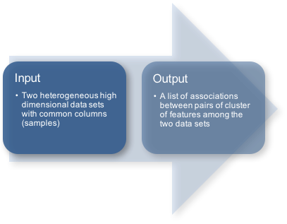
HAllA inputs:
Data in scientific studies often come paired in the form of two high-dimensional datasets, where the dataset X (with p features/rows and n samples/columns) are assumed to be p predictor variables (or features) measured on n samples that give rise to d response variables contained in the dataset Y (with d features/rows and n samples/columns). Note that column i of X is sampled jointly with column i of Y, so that X and Y are aligned.
HAllA output:
HAllA reports significant associations between clusters of related features ("block associations"). Each block association is characterized by a cluster from the first dataset, a cluster from the second dataset, and measures of statistical significance and effect size (p-value, q-value, and similarity score) for the cluster's component pairwise associations.
Support:
- Please direct questions to the HAllA support forum.
- For additional information, see the HAllA User Manual.
- Table of Contents
- Installation
- How to run
- Visualizing HAllA results
- Changing HAllA's default behavior
- Synthetic data experiments
pip install halla
Note: Please install the following R packages manually:
git clone https://github.com/biobakery/halla.git
cd halla
python setup.py develop
Other than Python (version >= 3.7) and R (version >= 3.6.1), install all required libraries listed in requirements.txt, specifically:
Requirements Python packages:
- jenkspy (version >= 0.1.5)
- Matplotlib (version >= 3.5.3)
- NumPy (version >= 1.19.0)
- pandas (version >= 1.0.5)
- PyYAML (version >= 5.4)
-
rpy2 (version >= 3.3.5) - Notes on installing
rpy2in macOS - scikit-learn (version >= 0.23.1)
- SciPy (version >= 1.5.1)
- seaborn (version >= 0.10.1)
- statsmodels (version >= 0.11.1)
- tqdm (>=4.50.2)
R packages:
# for MacOS - read the notes on installing rpy2:
#   specifically run 'env CC=/usr/local/Cellar/gcc/X.x.x/bin/gcc-X pip install rpy2'
#   where X.x.x is the gcc version on the machine **BEFORE** running the following command
HAllA requires as input two tab-delimited text files representing two paired datasets (sets of features) describing the same set of samples. Download the two demo datasets below and move them to your current working directory to get started with the tutorial:
These two files each contain 16 normally-distributed features measured from 100 samples (all synthetic data). Cluster structure was spiked into each dataset, and some clusters were forced to be associated to induce block association structure.
Next, run HAllA on the two demo input files, placing the output files in your current working directory under synthetic_output:
$ halla -x X_16_100.txt -y Y_16_100.txt -m spearman -o synthetic_output
HAllA uses Spearman's rank correlation as a default similarity measure for continuous data. If there is at least one categorical variable in either dataset, HAllA will shift to Normalized Mutual Information (NMI) as an alternative similarity measure. In either case, HAllA will then apply Benjamini-Hochberg FDR correction to the similarity measures' nominal p-values. Learn more about changing HAllA's default options in the exercises below.
The command above creates two primary output files:
sig_clusters.txtall_associations.txt
Let's examine these files individually, starting with sig_clusters.txt, which reports block associations between the two datasets' features:
$ column -t -s $'\t' synthetic_output/sig_clusters.txt | less -S
This yields: :
cluster_rank  cluster_X   cluster_Y   best_adjusted_pvalue
1             X12;X13     Y12;Y13     1.2567120809513244e-12
2             X14;X15     Y14;Y15     1.3331224180115239e-11
3             X9;X10;X11  Y9;Y10;Y11  4.025783938784645e-10
4             X0;X1;X2    Y0          7.360629458577536e-09
5             X6          Y6          5.580991792016541e-06
6             X3          Y3          1.5637124978622357e-05
7             X3;X4;X5    Y4;Y5       1.601935000755317e-05
8             X6;X7;X8    Y7          1.879154176502828e-05
9             X0;X1;X2    Y1          3.229563260817097e-05
10            X8          Y8          0.00044616349146898895
11            X2          Y2          0.0006213586345147157
12            X14;X15     Y6          0.002468944332992917
13            X4          Y3          0.003754984672983486
14            X6          Y3          0.035578246404989286
15            X7          Y6          0.03922861489400263
Now let's examine all_associations.txt, which reports the pairwise similarity scores for all features across the two datasets:
$ column -t -s $'\t' synthetic_output/all_associations.txt | less -S
This yields:
X_features  Y_features  association            p-values                q-values
X0          Y0          0.75875150060024       1.72514752935411e-10    7.360629458577536e-09
X0          Y1          0.47515006002400956    0.0004888172137947008   0.0039105377103576065
X0          Y2          0.16398559423769507    0.25514193499628157     0.6597609632227079
X0          Y3          0.12921968787515006    0.37112486503493036     0.7897491914951426
X0          Y4          0.18136854741896757    0.2074830356872076      0.5711360982357543
X0          Y5          0.18021608643457382    0.21043410218481773     0.5724099195863718
X0          Y6          -0.03279711884753902   0.8211191874364518      0.9721674283495674
X0          Y7          -0.25330132052821125   0.07591776313339742     0.2858080494433785
X0          Y8          0.0052340936374549825  0.9712227578351469      0.9750314745325396
X0          Y9          -0.06948379351740695   0.6315987410557464      0.9362240451170357
X0          Y10         -0.12864345738295319   0.37327989129262595     0.7897491914951426
X0          Y11         0.018103241296518604   0.9006963927911024      0.9721674283495674
X0          Y12         -0.3153421368547419    0.025703636157753368    0.13428838482418087
X0          Y13         -0.12432172869147658   0.3896805398051253      0.8110424243098543
X0          Y14         -0.2053781512605042    0.15248320921458566     0.4703096573365534
X0          Y15         -0.19241296518607443   0.18066815479989504     0.5255800866906037
X1          Y0          0.48600240096038416    0.00034616222922012244  0.002953917689345045
X1          Y1          0.617671068427371      1.76616740825935e-06    3.229563260817097e-05
X1          Y2          0.25032412965186074    0.07954656945356582     0.2951293011610558
X1          Y3          0.2844177671068427     0.0453037212343839      0.19329587726670464
X1          Y4          0.23755102040816325    0.09668797802947016     0.3486214419090755
X1          Y5          0.28297719087635054    0.04645373054759285     0.19495336098661917
X1          Y6          -0.0811044417767107    0.5755384891432878      0.9094929211153189
X1          Y7          -0.09656662665066026   0.5046953555630573      0.89287834235078
X1          Y8          -0.049219687875150055  0.7342792173788053      0.9652446357780742
X1          Y9          0.15034813925570228    0.29733245851279005     0.7180859375403231
X1          Y10         0.058439375750300115   0.6868585612891065      0.9402983512834827
:
- What is the pairwise similarity score between feature X9 and feature Y11 in association number 3? How does this score compare with the similarity score given for association number 3?
- What is the pairwise similarity score between X15 and Y6? How does this compare to the strength of association considered above? How is this difference reflected in the p-value and q-value of the test for these two features?
Here we will consider subsets of a published dataset (Morgan et al., Genome Biol, 2015) that combined 1) 16S rRNA amplicon sequencing of the human gut microbiome (64 taxa) and 2) Affymetrix microarray screens of colonic RNA expression (100 genes) across 204 patients with ulcerative colitis. We will refer to this as the "pouchitis dataset."
The purpose of this study was to associate human genes and microbial taxa with the recurrence of inflammation following ileal resection surgery (a surgical procedure in ulcerative colitis that involves removing of the large intestine and rectum and attaching the lowest part of the small intestine to a hole made in the abdominal wall to allow waste to leave the body).
Download the paired, subsampled OTU and gene expression datasets:
Run HAllA on these datasets: :
$ halla -x otu_299.txt -y gene_200.txt -o pouchitis_output -m spearman --fdr_alpha 0.05
Note the addition of the --fdr_alpha flag: this defines the target FDR, here 0.05, i.e. the expected fraction of false positive reports among returned significant associations.
hallagram is a utility included with HAllA for visualizing the method's discovered block associations as inspected in text form above. Run hallagram as follows (use hallagram -h for help with plot options):
$ hallagram \
    -i synthetic_output/ \
    --cbar_label 'Pairwise Spearman' \
    --x_dataset_label X \
    --y_dataset_label Y \
    --block_border_width 2
Open the file hallagram.png in the synthetic_output directory, which should look like this:

- How many features are involved in the largest association in the figure? How many pairwise associations does this cluster association represent? Does it appear as though the pairwise associations are reasonably homogeneous in terms of their strength?
- Are there any pairs of clusters with a significant negative association?
- Do you think that HAllA's approach improved statistical power in this scenario? How would power be different if all X and Y features were compared individually?
Let's try some of the other hallagram options using the pouchitis dataset (gut OTUs and host gene expression):
$ hallagram \
    -i pouchitis_output/ \
    --cbar_label 'Pairwise Spearman' \
    --x_dataset_label 'Microbial OTUs' \
    --y_dataset_label 'Gene expression' \
    -n 30 \
    --block_border_width 2
What are these new options doing?
-
--x_dataset_labelassigns a label to the X dataset features (rows) -
--y_dataset_labelassigns a label to the Y dataset features (cols) -
-nor--block_numsets the number of best-ranked blocks (sorted by similarity score) to be included in the figure.
And here is the resulting figure:

- How would you interpret association number 10?
- How would your answers regarding the previous hallagram change here?
Additionally, we can investigate specific associations within clusters. The hallagnostic utility generates a lattice plot showing the pairwise associations between microbiome features and metadata for each significant cluster. We can use -n 8 to specify that we only want diagnostic plots for the first 8 blocks.
Let's explore diagnostic plots for the pouchitis data:
$ hallagnostic -i pouchitis_output/ -n 8
A directory called diagnostic will be generated in the pouchitis_output/ containing the diagnostic plots. The plot for the first cluster is called association_1.png (shown below). The diagonal entries show empirical cumulative density plots for each feature in the cluster. The off-diagonal plots show pairwise feature plots for each pair of features in the cluster. This can be helpful for distinguishing between real associations driven by consistent trends and spurious associations driven by outliers.

One of the most important settings in HAllA is the expected false negative rate (FNR) for block associations (--fnr_thresh). The default setting of this parameter is 0.2, meaning that a block of associations will be accepted if at least 80% of its component pairwise associations are statistically significant (thus treating the remaining 0-20% of non-significant associations in the block as probable false negatives).
The fact that these negative associations are clustered among otherwise significantly associated features from their respective datasets boosts our confidence that they too are associated (a form of prediction based on "guilt-by-association" logic). A modest expected false negative rates thus serves to improve HAllA's sensitivity without compromising specificity (excess false positives).
Let's try a HAllA run on the synthetic data after increasing the FNR threshold to 0.3:
$ halla -x X_16_100.txt -y Y_16_100.txt \
    -o synthetic_output_fnr_thresh_30_percent \
    -m spearman --fnr_thresh 0.3
Then rebuild the HAllAgram for the modified run:
$ hallagram \
    -i synthetic_output_fnr_thresh_30_percent \
    --cbar_label 'Pairwise Spearman' \
    --x_dataset_label X \
    --y_dataset_label Y \
    --block_border_width 2
Which looks like:

- Compare this hallagram to the one generated using the default FNR threshold of 0.2 (
synthetic_output/hallagram.png). What has changed?
HAllA uses robust similarity measures to build hierarchical clusters within datasets and to find associations between datasets. By default, HAllA uses Spearman Correlation for purely continuous datasets and Normalized Mutual Information (NMI) for datasets containing categorical variables. You can use the -m flag to manually specify a similarity measure for a given HAllA run.
Let's try a HAllA run on the synthetic data using mutual information as an alternative to Spearman Correlation for quantifying association strength.
$ halla -x X_16_100.txt -y Y_16_100.txt \
    -o synthetic_output_mi \
    -m mi
- What has changed in the output files?
HAllA performs many statistical tests when initially constructing the all-against-all similarity matrix. These must be subjected to some form of multiple hypothesis testing correction to avoid reporting large numbers of false positive associations. By default, HAllA follows a false discovery rate (FDR) control approach using the Benjamini-Hochberg (BH) method. Other approaches and methods available in Python's statsmodels module can also be used in HAllA.
Let's try a HAllA run on the synthetic data using the Bonferroni method for family-wise error rate control:
$ halla -x X_16_100.txt -y Y_16_100.txt \
    -o synthetic_output_bonferroni \
    -m spearman \
    --fdr_method bonferroni
- What has changed in the output files?
HAllA uses a hierarchical approach for block association discovery on top of an existing all-against-all (AllA) association matrix. To skip the block association step, you can run HAllA with the --alla flag. Let's try this approach on the synthetic data:
$ halla -x X_16_100.txt -y Y_16_100.txt \
    -o synthetic_output_alla \
    -m spearman \
    --alla
- What has changed in the output files?
In this section, we'll use another HAllA utility, halladata, to generate synthetic datasets with pre-defined feature and block association structure. We will then attempt to recover those associations using HAllA with different settings.
The following command generates a pair of datasets with 32 mixed (categorical and continuous) features "measured" over 100 samples. Continuous features are sampled uniformly and categorical features are balanced.
$ halladata -n 100 -xf 32 -yf 32 -a mixed -o halla_data_f32_n100_mixed
Try analyzing these data by forcing HAllA to use Spearman correlation:
$ halla \
    -x halla_data_f32_n100_mixed/X_mixed_32_100.txt \
    -y halla_data_f32_n100_mixed/Y_mixed_32_100.txt \
    -o halla_output_f32_n100_mixed \
    -m spearman
- What happens and why?
Now run HAllA with the NMI similarity measure:
$ halla \
    -x halla_data_f32_n100_mixed/X_mixed_32_100.txt \
    -y halla_data_f32_n100_mixed/Y_mixed_32_100.txt \
    -o halla_output_f32_n100_mixed \
    -m nmi
Let's now generate synthetic continuous data with a linear relationship between and within datasets to see how Spearman Correlation versus NMI compare in their ability to recover the associations.
$ halladata -n 50 -xf 32 -yf 32 -a line --o halla_data_f32_n50_line
Run HAllA with the default similarity metric (Spearman as all data are continuous):
$ halla \
    -x halla_data_f32_n50_line/X_line_32_50.txt \
    -y halla_data_f32_n50_line/Y_line_32_50.txt \
    -o halla_output_f32_n50_line_spearman \
    -m spearman
Then build a HAllAgram:
$ hallagram \
    -i halla_output_f32_n50_line_spearman \
    --cbar_label 'Pairwise Spearman' \
    --x_dataset_label X --y_dataset_label Y \
    --block_border_width 2
Now repeat these two steps using NMI as a similarity measure (which will implicity discretize our simulated continuous features):
$ halla \
    -x halla_data_f32_n50_line/X_line_32_50.txt \
    -y halla_data_f32_n50_line/Y_line_32_50.txt \
    -o halla_output_f32_n50_line_nmi \
    -m nmi

$ hallagram \
    -i halla_output_f32_n50_line_nmi \
    --cbar_label 'Pairwise NMI' \
    --x_dataset_label X \
    --y_dataset_label Y \
    --block_border_width 2
- How do the two runs' HAllAgrams differ? What causes these differences?