9 ‐ Audio‐based Processes

For complete documentation see Audio Analysis on the docs site.

---

Sound can be looked at too. A waveform shows how loud the recording is from moment to moment, which for a dance session mostly means footsteps, breath, music and talk. A spectrogram adds what the sound is made of—low rumble at the bottom, hiss and consonants at the top—so a drum hit and a spoken word, equally loud, look nothing alike. These methods draw sound so it can sit on the same page as the movement.

Audio analysis methods work on both mv.audio (from an MgVideo) and MgAudio (for audio-only files). All methods return an MgFigure and save a PNG alongside the source file. Every method also accepts a title argument for the figure heading.

import musicalgestures as mg

# From a video file
mv = mg.MgVideo('/path/to/video.avi')
audio = mv.audio

# Or load an audio file directly
audio = mg.MgAudio('/path/to/audio.mp3')

Waveform

A waveform plots audio amplitude over time. It gives a quick overview of loudness and silence, and it is the natural first look at any recording.

waveform = audio.waveform()
waveform.show()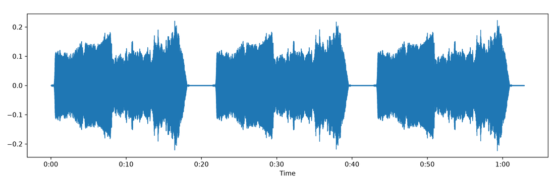

Waveform: audio amplitude over time, giving a quick overview of loudness and silence.

Pass raw=True to skip librosa post-processing and plot the raw sample values:

waveform = audio.waveform(raw=True)

Set colored=True to render a frequency-coloured waveform, in the style of freesound.org. This draws the amplitude envelope with colour representing the spectral centroid, so bright and dull passages separate at a glance:

colored = audio.waveform(colored=True)
colored = audio.waveform(colored=True, cmap='jet')

Any Matplotlib colormap name is accepted for cmap.

Spectrogram

A mel spectrogram plots frequency content over time and is more informative than a waveform for most audio. Two sounds of equal loudness that look identical in the waveform look nothing alike here.

spectrogram = audio.spectrogram()
spectrogram.show()
spectrogram = audio.spectrogram(raw=True)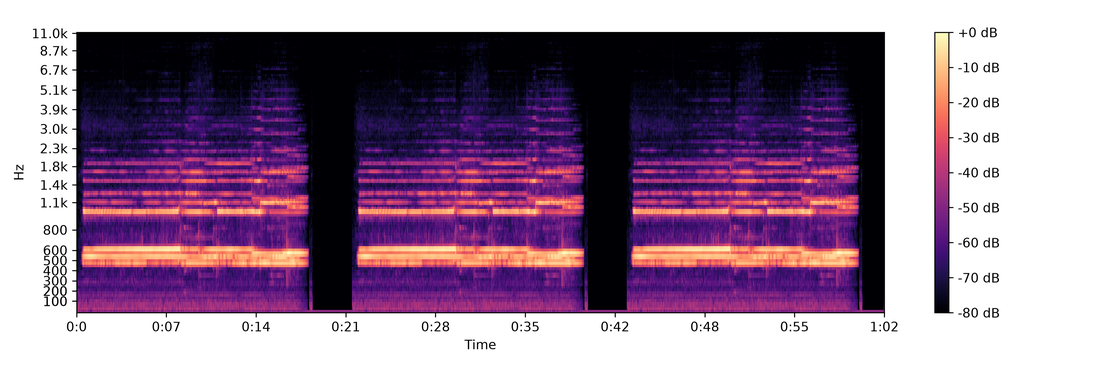

Mel spectrogram: frequency content over time, more informative than a waveform for most audio.

MFCC

Mel-frequency cepstral coefficients compactly describe the spectral envelope (the measured counterpart of timbre) over time and are widely used as audio features.

mfcc = audio.mfcc()
mfcc = audio.mfcc(n_mfcc=20)
mfcc.show()

coeffs = audio.mfcc(autoshow=False).data['mfcc']   # numpy array (n_mfcc, frames)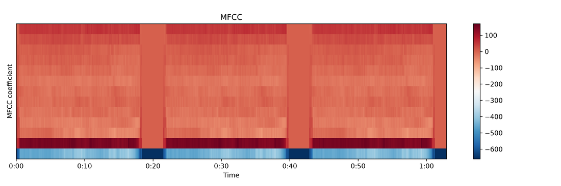

MFCC: mel-frequency cepstral coefficients describing the spectral envelope, the measured counterpart of timbre, over time.

Chromagram

A chromagram maps audio energy onto the 12 pitch classes (C, C#, D, …, B) over time. It is useful for analysing harmony, chord progressions, and key.

chroma = audio.chromagram()
chroma.show()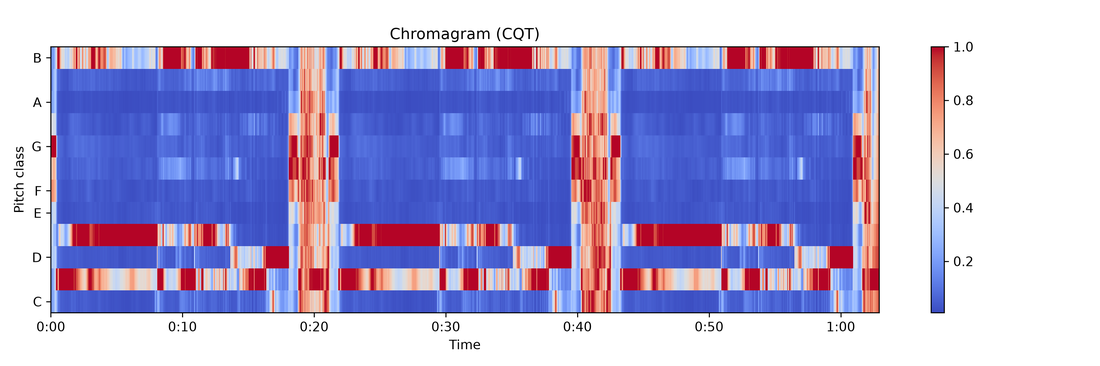

Chromagram: audio energy mapped onto the 12 pitch classes over time, useful for harmony, chord progressions, and key.

Three algorithms are available via chroma_type:

chroma_type	Algorithm	Best for
'cqt' (default)	Constant-Q Transform	Music with low-frequency content
'stft'	Short-Time Fourier Transform	Fast computation
'cens'	Chroma Energy Normalised Statistics	Robustness to timbre and dynamics

chroma_cqt  = audio.chromagram(chroma_type='cqt')
chroma_stft = audio.chromagram(chroma_type='stft')
chroma_cens = audio.chromagram(chroma_type='cens')

You can also control normalisation and colormap:

chroma = audio.chromagram(norm=2, cmap='viridis')   # L2 norm, viridis colormap
chroma = audio.chromagram(norm=None)                 # no normalisation

The chroma array (shape 12 × frames) is available in the returned MgFigure:

mgf = audio.chromagram()
chroma_data = mgf.data['chroma']   # numpy array, shape (12, n_frames)

Harmonic Percussive Source Separation (HPSS)

HPSS uses median filtering to separate the harmonic and percussive components of the audio. Separating a drum track from sustained tones makes both easier to read. An optional residual component captures sounds between the two.

hpss_fig = audio.hpss()
hpss_fig = audio.hpss(residual=True)
hpss_fig.show()

Tempogram

A tempogram estimates tempo by analysing onset strength over time using FFT, giving a view of rhythmic periodicity. Where a spectrogram shows what the sound is made of, a tempogram shows when things happen and how regularly.

tempogram = audio.tempogram()
tempogram.show()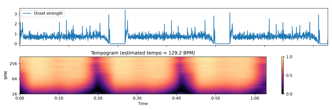

Tempogram: rhythmic periodicity from onset strength over time, with an onset-strength panel above and the estimated tempo in the title.

By default the figure includes an onset-strength panel above the tempogram. Pass onset_strength=False for just the tempogram in a single panel (the same size as the spectrogram/chromagram):

audio.tempogram(onset_strength=False).show()

The tempogram is drawn with a colourbar (matching the chromagram), and the estimated tempo is shown rounded to one decimal in the plot title, e.g. Tempogram (estimated tempo = 112.3 BPM).

Tempo and beat tracking

tempo() estimates the tempo and beat positions and renders the waveform with beat markers. Numeric results are in the returned figure's .data:

t = audio.tempo()
t.show()

print(t.data['tempo'])            # BPM
print(t.data['beat_times'])       # beat positions (s)
print(t.data['beat_regularity'])  # 1.0 = perfectly even beats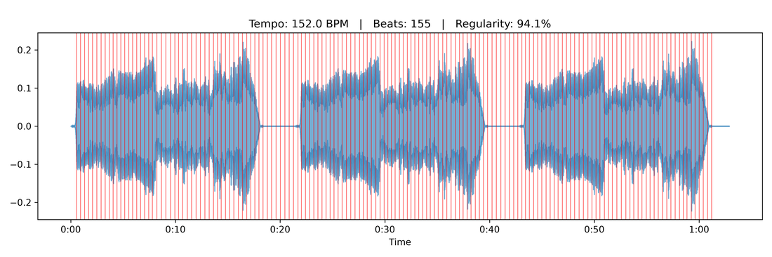

Tempo: the waveform with detected beat markers; numeric tempo, beat times, and regularity are in the figure's .data.

Available .data keys: tempo, beat_times, ibi (inter-beat intervals), beat_regularity, beat_phases, deviations_s, R_beat, mu_beat, T_fit, t0_fit, p_rayleigh.

Beat statistics

beat_statistics() fits an ideal isochronous grid to the detected beats and visualises how each beat deviates from it, in a polar phase histogram plus a millisecond-deviation time series. This shows whether a performer rushes, drags, or keeps steady time. It requires at least four detected beats.

stats = audio.beat_statistics()
stats.show()

The polar plot shows the mean resultant vector length R (concentration of timing) and a Rayleigh-test p-value (p small = significantly consistent timing).

On an MgVideo, beat_statistics() defaults to source='motion': it runs the timing analysis on onsets detected in the quantity of motion. This is the key difference from video.audio.beat_statistics(), which always analyses the audio track. Pass source='audio' to analyse the audio track from the video instead:

mv = mg.MgVideo('dance.mp4')
mv.beat_statistics()                   # default — onsets in the quantity of motion
mv.beat_statistics(source='motion')   # explicit; same as the default
mv.beat_statistics(source='audio')    # the audio track instead
mv.audio.beat_statistics()            # the audio track (always audio)

source='motion' returns an MgFigure whose .data holds the motion tempo, beat times, regularity, and phase deviations, the same fields as the audio version.

Self-Similarity Matrix (SSM)

Audio SSMs compare feature frames against each other to reveal repeating structure (verse/chorus, loops, etc.). Supported features are 'spectrogram', 'chromagram', and 'tempogram'.

spectrossm = audio.ssm(features='spectrogram')
chromassm  = audio.ssm(features='chromagram', cmap='magma', norm=2)
spectrossm.show()

SSMs can also be computed on visual features from MgVideo; see Video‐based Processes.

Audio descriptors

descriptors() plots five spectral features over time in a single figure:

• RMS energy (the measured correlate of loudness)
• Spectral flatness (noisiness vs. tonality)
• Spectral centroid (brightness)
• Spectral bandwidth (frequency spread)
• Spectral rolloff (at 1% and 99% of total energy)

descriptors = audio.descriptors()
descriptors.show()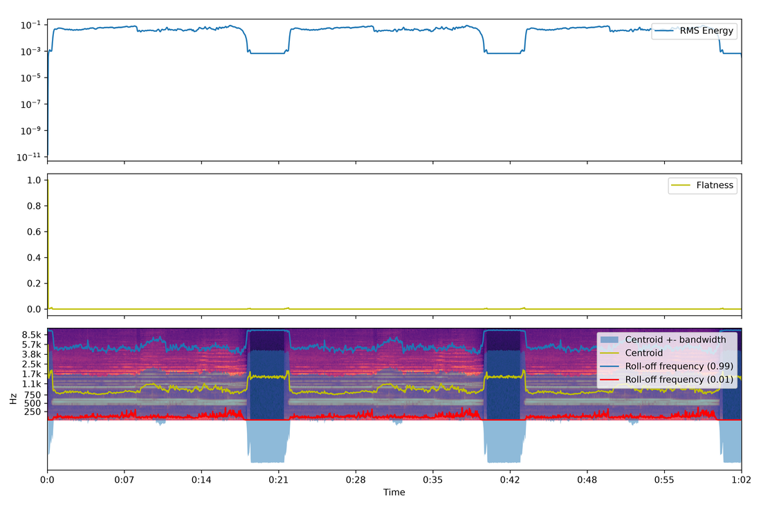

Audio descriptors: RMS energy, spectral flatness, centroid, bandwidth, and rolloff plotted over time in a single figure.

Set save_data=True to also write the per-frame descriptor time series to disk (csv/tsv/txt), mirroring motiondata:

audio.descriptors(save_data=True, data_format='csv')   # or 'tsv' / 'txt' / ['csv','txt']
# writes <name>_descriptors.csv with columns:
# Time, RMS, Centroid, Bandwidth, Rolloff, RolloffMin, Flatness

Descriptors can be overlaid on motion plots by passing audio_descriptors=True to motionplots():

mv.motionplots(audio_descriptors=True)

Sound together with movement

When the audio and the movement come from the same performer (e.g. a dancer who is also the sound source), several MgVideo methods compare the sound with the motion directly: tempo_similarity(), phase_synchrony(), structure_comparison(), motion_audio_coupling(), and dynamics_coupling(). They live on MgVideo because they need both tracks, and they are covered with example figures in Video‐based Processes.

Related: MgVideo.sonomotiongram() turns a motiongram back into sound (returns an MgAudio).