Tutorial Build a Model

Tutorial · Build a Model

GUI Tutorial · Chapter 3 of 4 — the hands-on half of a complete study: from a raw µCT image stack to a meshed, material-assigned nerve with a cuff electrode. Chapter 4, Simulate & Export, then solves the field and runs the fibers.

The example project is a human extruded nerve.

---

6.1 Create the project

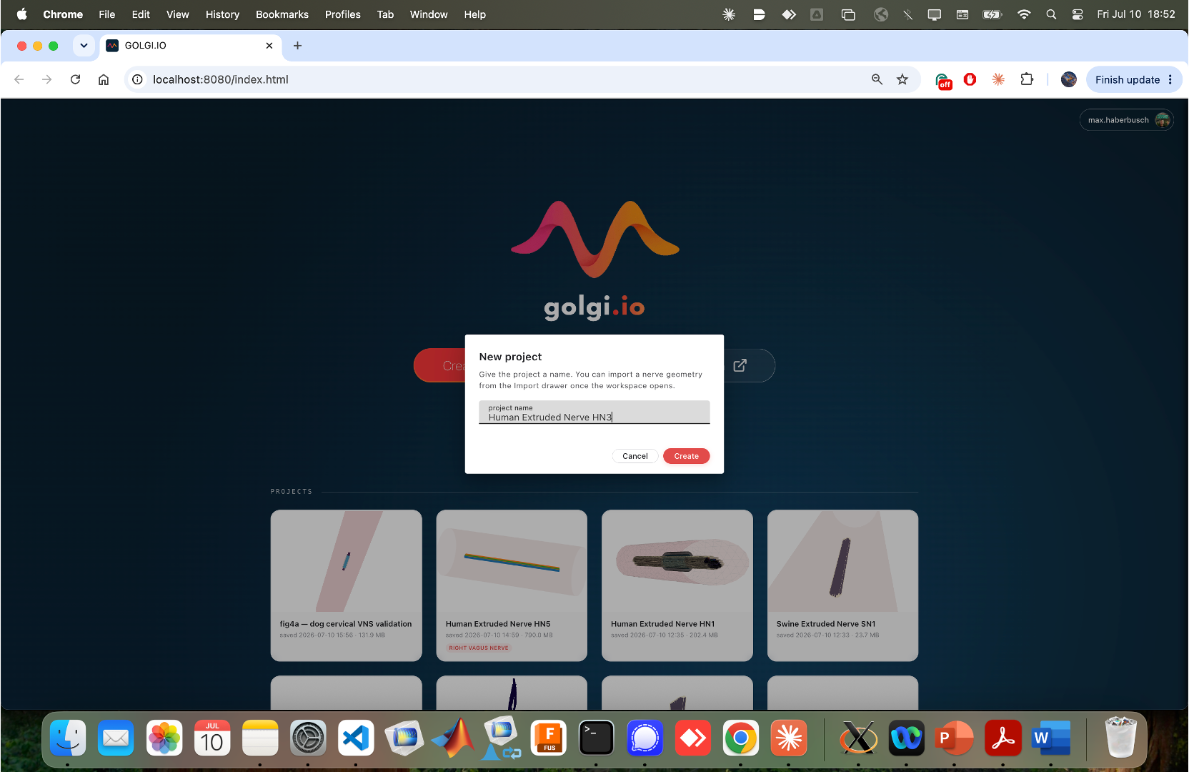
From the dashboard click Create new project (or, in the workspace, FILE → Close project and start fresh). The New project dialog asks only for a project name; you will import the geometry afterwards from the Import drawer once the workspace opens. Type a descriptive name (here, Human Extruded Nerve HN3) and click Create.

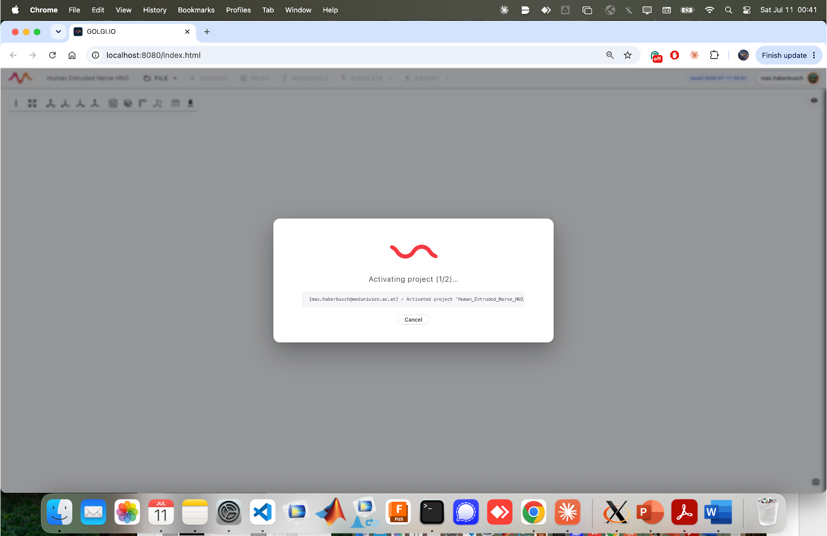
golgi activates the new project. A brief "Activating project…" dialog with a log confirms the workspace is being prepared.

---

6.2 Segment a µCT slice and extrude it as a nerve

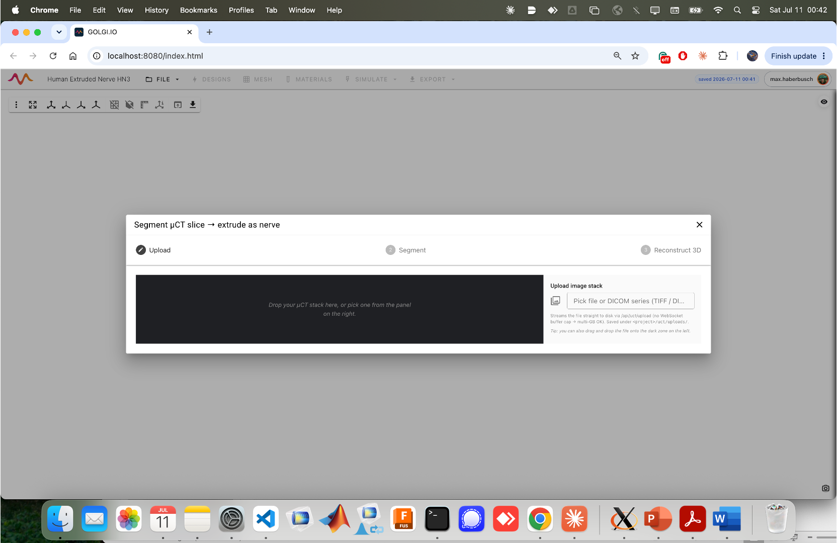
With an empty project open, choose FILE → Segment µCT slice…. This opens the three-step wizard Segment µCT slice → extrude as nerve, whose steps are Upload → Segment → Reconstruct 3D. (The deeper reference for this stage is Geometry Import & Segmentation.)

Step 1 — Upload

Drag a µCT stack onto the dark drop zone, or use Pick file or DICOM series (TIFF / DICOM…) on the right. The file is streamed straight to disk, so multi-gigabyte stacks are fine.

Step 2 — Segment

Once the stack loads, the Segment step shows the current slice on the left and the controls on the right. The header reports the stack dimensions (e.g. 26 frames · 2864 × 2864 · dtype int16).

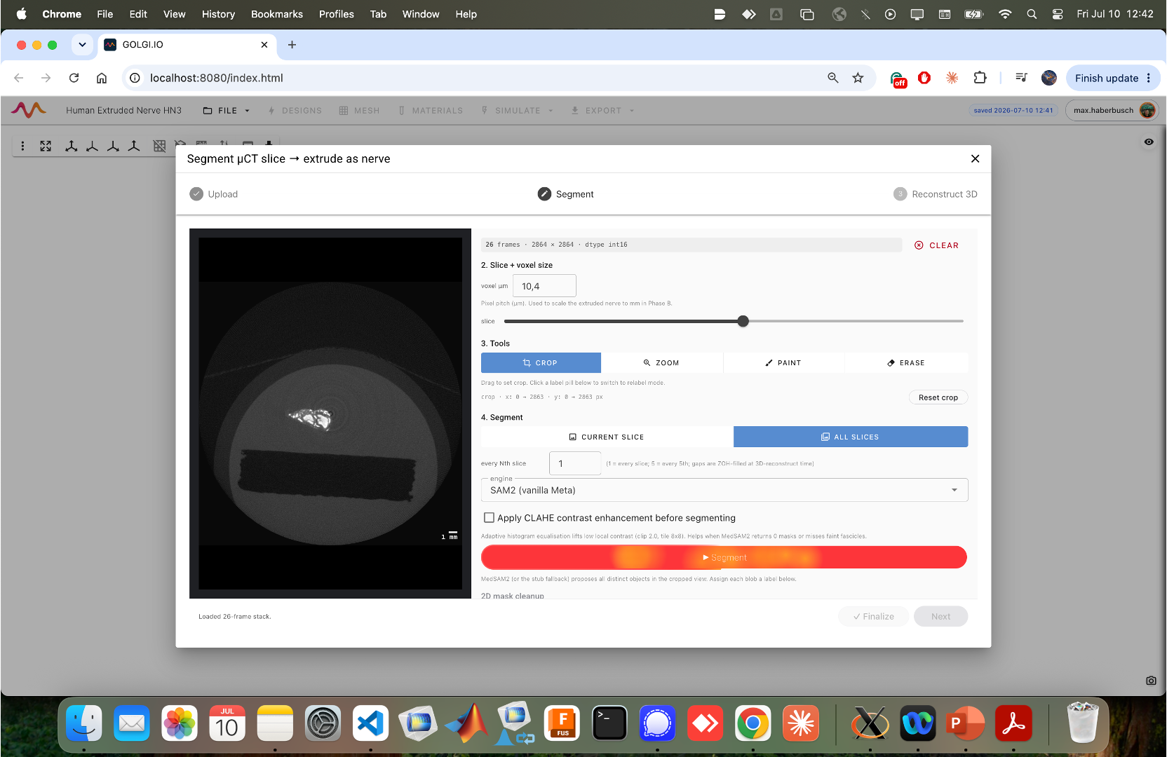
Work top-to-bottom through the controls:

• 2. Slice + voxel size. Enter the voxel µm (pixel pitch, e.g. 10.4). This scales the extruded nerve into millimeters later. The slice slider scrubs through the stack.
• 3. Tools. CROP (drag a box to restrict the working region), ZOOM, PAINT and ERASE (manual mask touch-ups). Reset crop clears the crop. Cropping tightly around the nerve, as below, makes the automatic segmentation faster and cleaner.

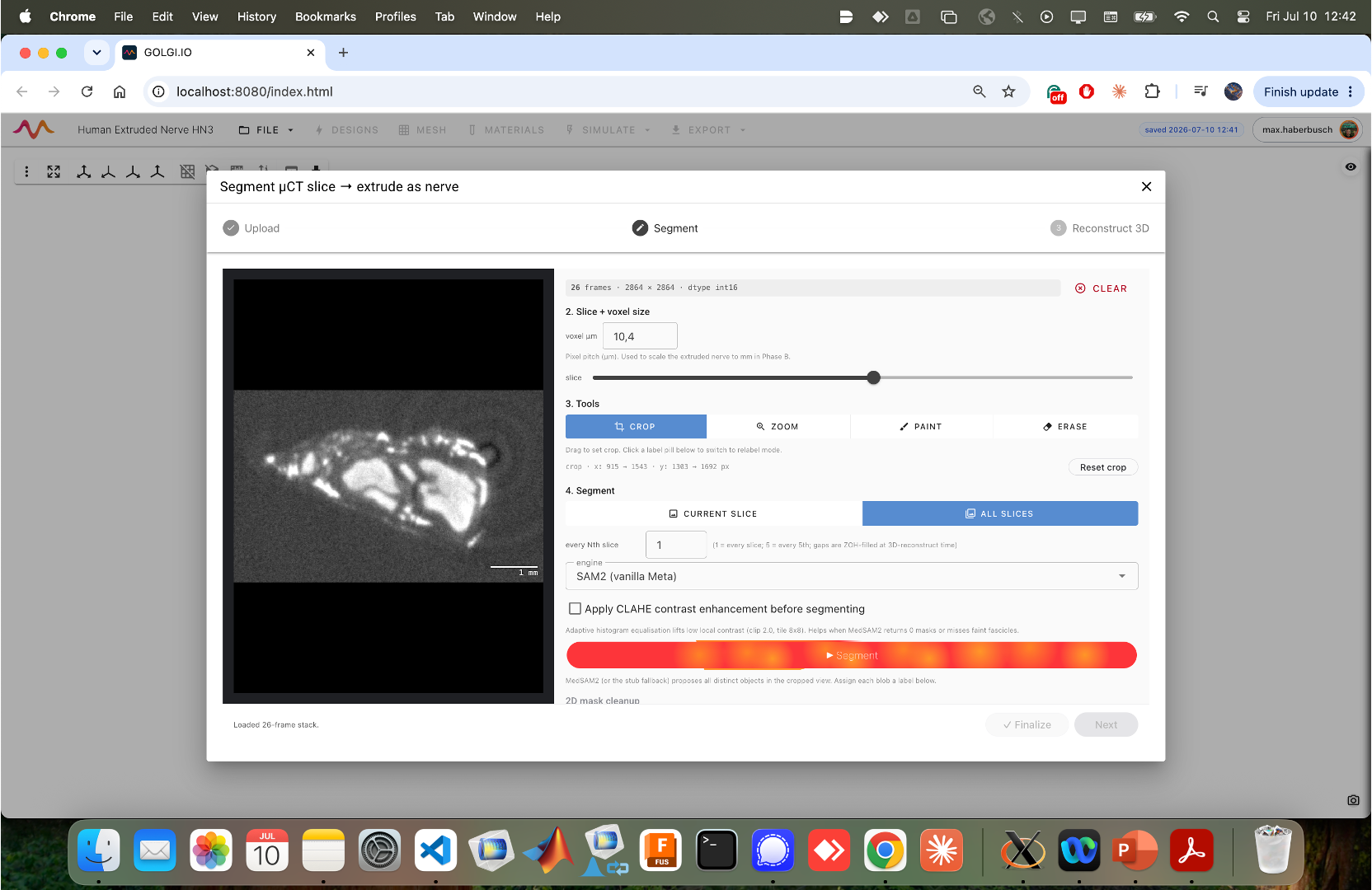
• 4. Segment. Choose whether to segment the CURRENT SLICE or ALL SLICES, set every Nth slice (1 = every slice; higher values sample sparsely and 3-D reconstruction fills the gaps), and pick the segmentation engine (e.g. SAM2 (vanilla Meta) — a general-purpose segment-anything model). Tick Apply CLAHE contrast enhancement before segmenting to lift local contrast if the model misses faint fascicles. Click ► Segment.

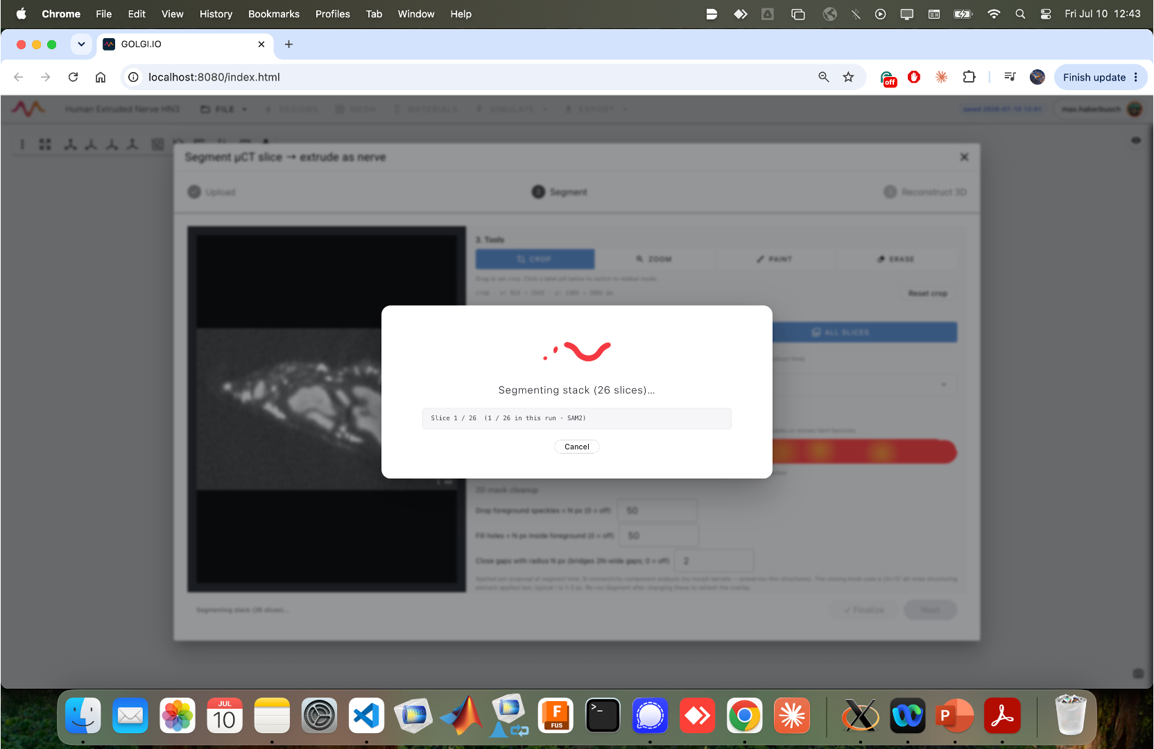
When you segment the whole stack, a progress dialog reports which slice is being processed ("Segmenting stack (26 slices)…").

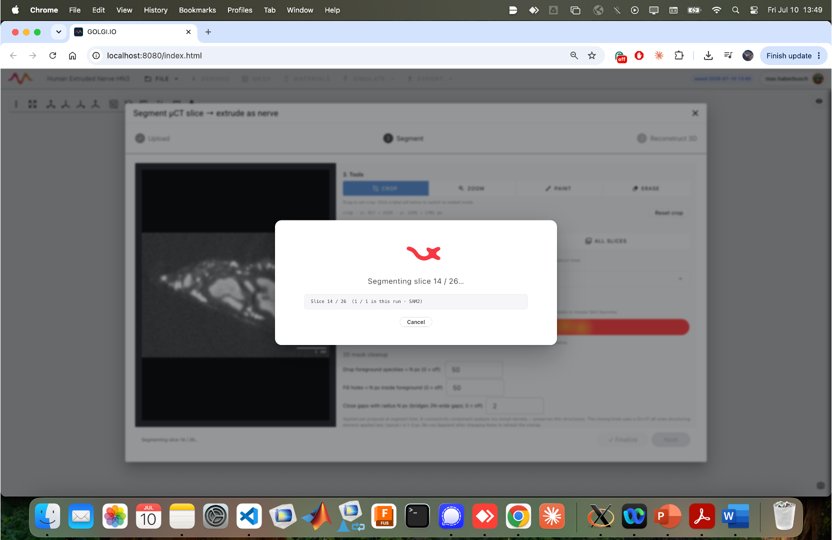
Individual-slice runs show a similar per-slice progress readout.

• 2D mask cleanup. After segmentation, tidy the masks: Drop foreground speckles < N px, Fill holes < N px inside foreground, and Close gaps with radius N px (bridges thin gaps). These morphological operations are applied per slice.
• 4b. Propagate from keyframes. For a stack, label a few good slices as keyframes (MARK KEYFRAME) and use ► Propagate from keyframes — SAM2 treats the z-stack as video frames and fills the rest forward and backward.
• 5. Assign labels. Each detected blob must be tagged. Pick the active label — Fascicle, Background, Epineurium or None — then click a colored mask in the preview to assign it. In the panel, each blob (#0, #1, …) shows its pixel area and centroid and a row of buttons (FASC., BG, EPI, NONE). Here the green region is a fascicle, the blue interior detail belongs to it, and the red rim is epineurium.

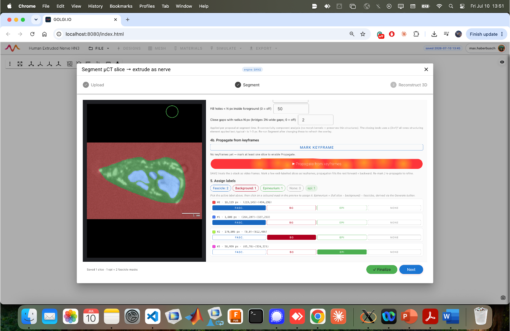
Click Finalize (saves the labelled slice) and then Next to move on.

Step 3 — Reconstruct 3D

The Reconstruct 3D step lofts the labelled 2-D slices into surfaces and shows the extruded nerve in an interactive preview, alongside a Mesh quality (per surface) panel with a histogram of triangle quality (q_radius_ratio) for each surface (epineurium and each fascicle). Use Show edges and Colour by mesh quality to inspect the surfaces, and Reset camera to reframe. The footer reports the STL files written (e.g. "Wrote 4 STL files").

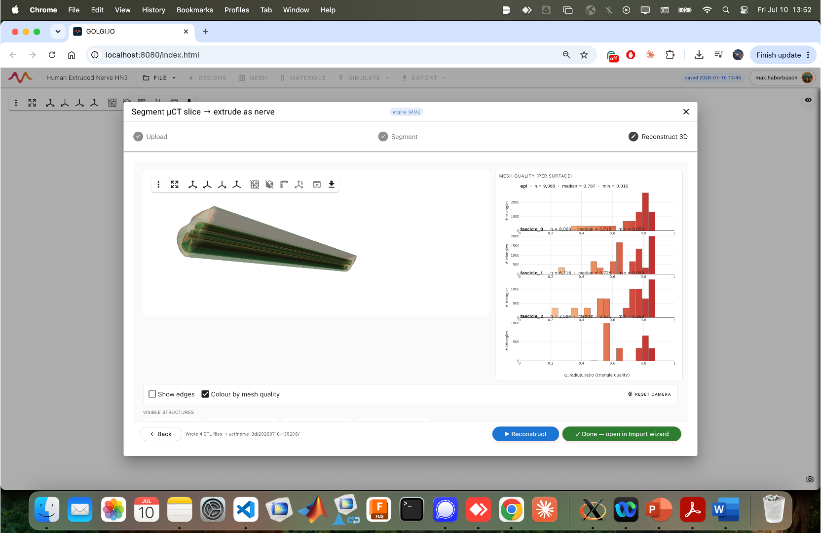
Click Reconstruct to (re)build, then Done — open in Import wizard to hand the geometry to the nerve setup wizard.

---

6.3 Set up the nerve, fibers and surrounding muscle

The Set up nerve wizard turns the reconstructed geometry into a simulation-ready nerve. Its steps are 1. Load nerve → 2. Endoneurium → 3. Fibers → 4. Muscle.

Step 1 — Load nerve

Choose the geometry source: STL surface (a single closed mesh from disk), Golgi µCT bundle (the bundle you just reconstructed), or Histology bundle. Pick the bundle from the Bundle dropdown — its label encodes the contents (e.g. epi + 3 fascicles · slice 13 · 50.00 mm extrude).

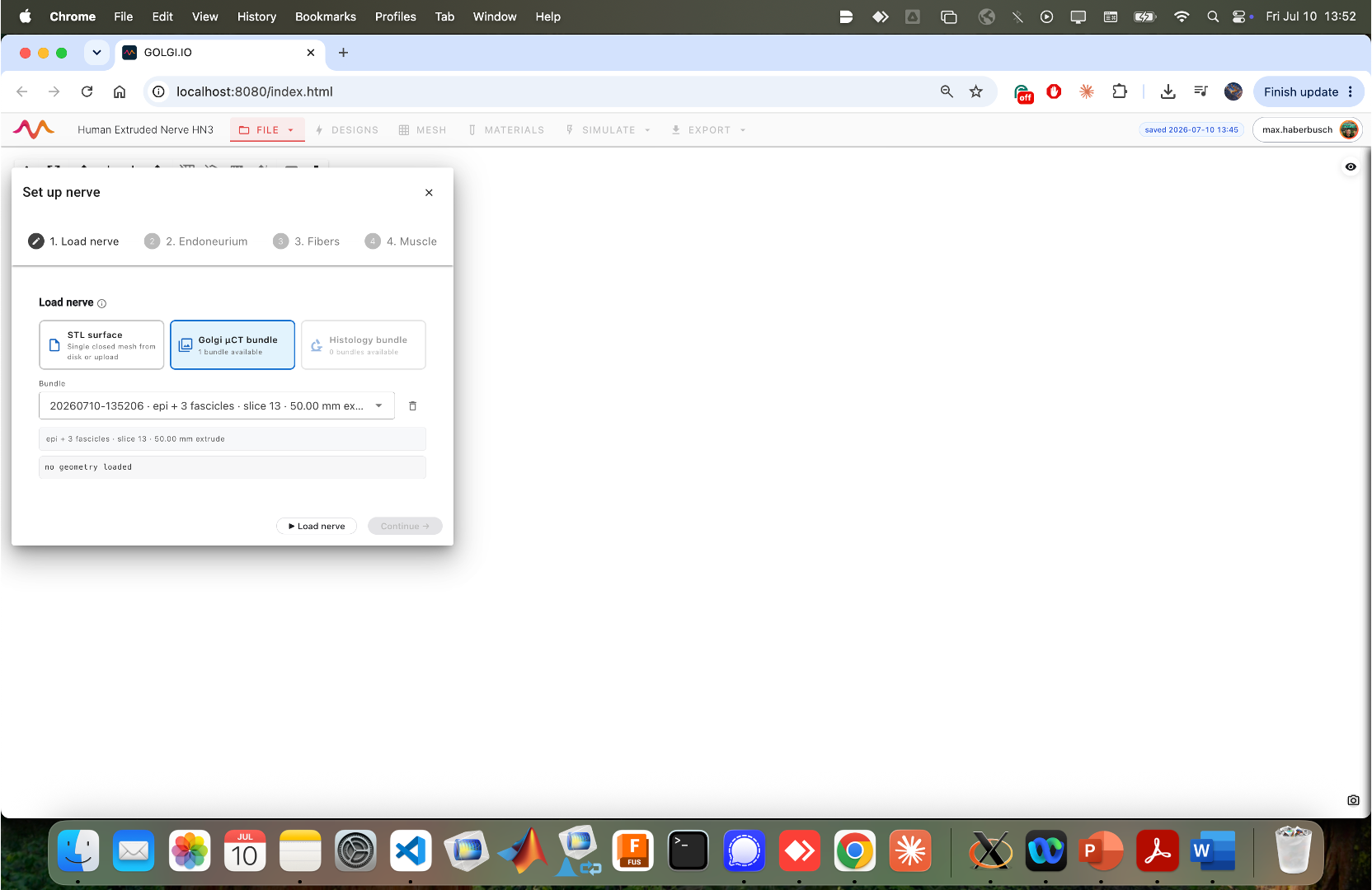
Click ► Load nerve. golgi reports the loaded geometry — point/triangle counts, bounding box, watertightness, open edges, non-manifold edges — and shows a Surface mesh quality histogram. A clean load reports watertight: yes with zero open or non-manifold edges. Use ✕ Remove loaded nerve to start over, or Continue → to proceed.

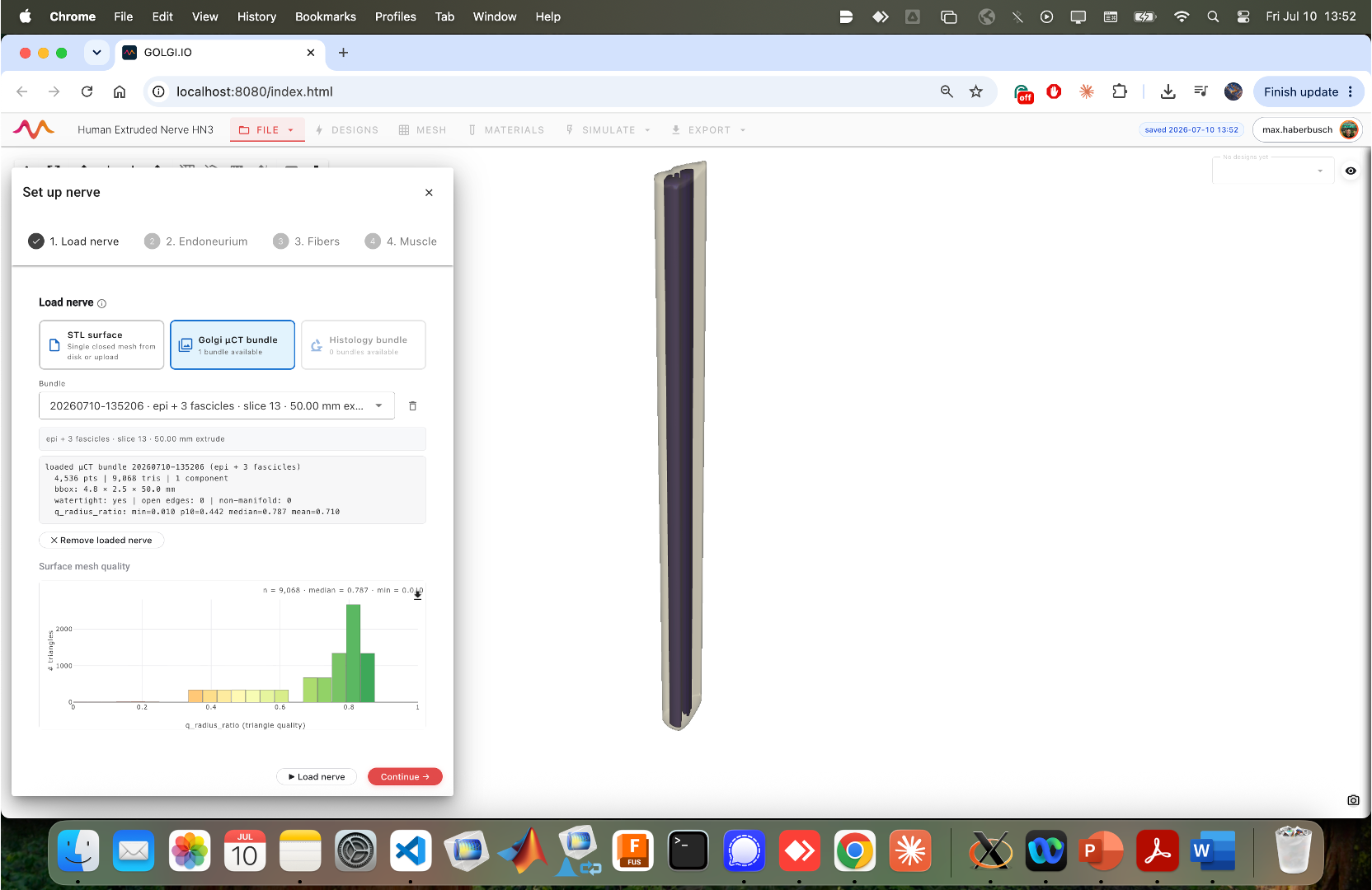
Step 2, Endoneurium, defines the intra-fascicular (endoneurial) compartment used by the field solve. In this example it is left at its defaults; advance through it with Continue →.

Step 3 — Fibers

The Fibers step generates axon trajectories inside the nerve. Set the Number of fiber seeds (e.g. 100), optionally tick Auto-detect branches (golgi finds distinct fascicle branches and distributes fibers among them), and pick a Generation method (e.g. Axial extrude, which extrudes seeds straight along the nerve axis). Click ► Generate fibers; the header confirms how many trajectories were produced (e.g. "101 trajectories generated").

The Branch summary table lists per-branch fiber counts and trajectory-length statistics (mean, min, max, std in millimetres). Here fibers split across Branch 0, Branch 1 and Branch 2. See Fiber Populations & Trajectories for the seeding and branch-detection details.

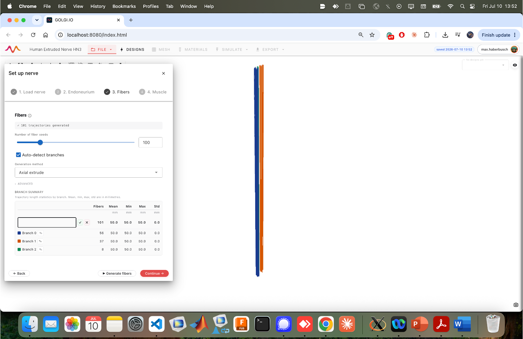
Click Continue →.

Step 4 — Muscle

The Muscle step wraps the nerve in a surrounding muscle/tissue cylinder, which acts as the volume conductor around the electrode. Set Radial padding and Axial padding (both in mm, e.g. 10) to control how much tissue surrounds the nerve. Click ► Generate muscle to preview, then Done.

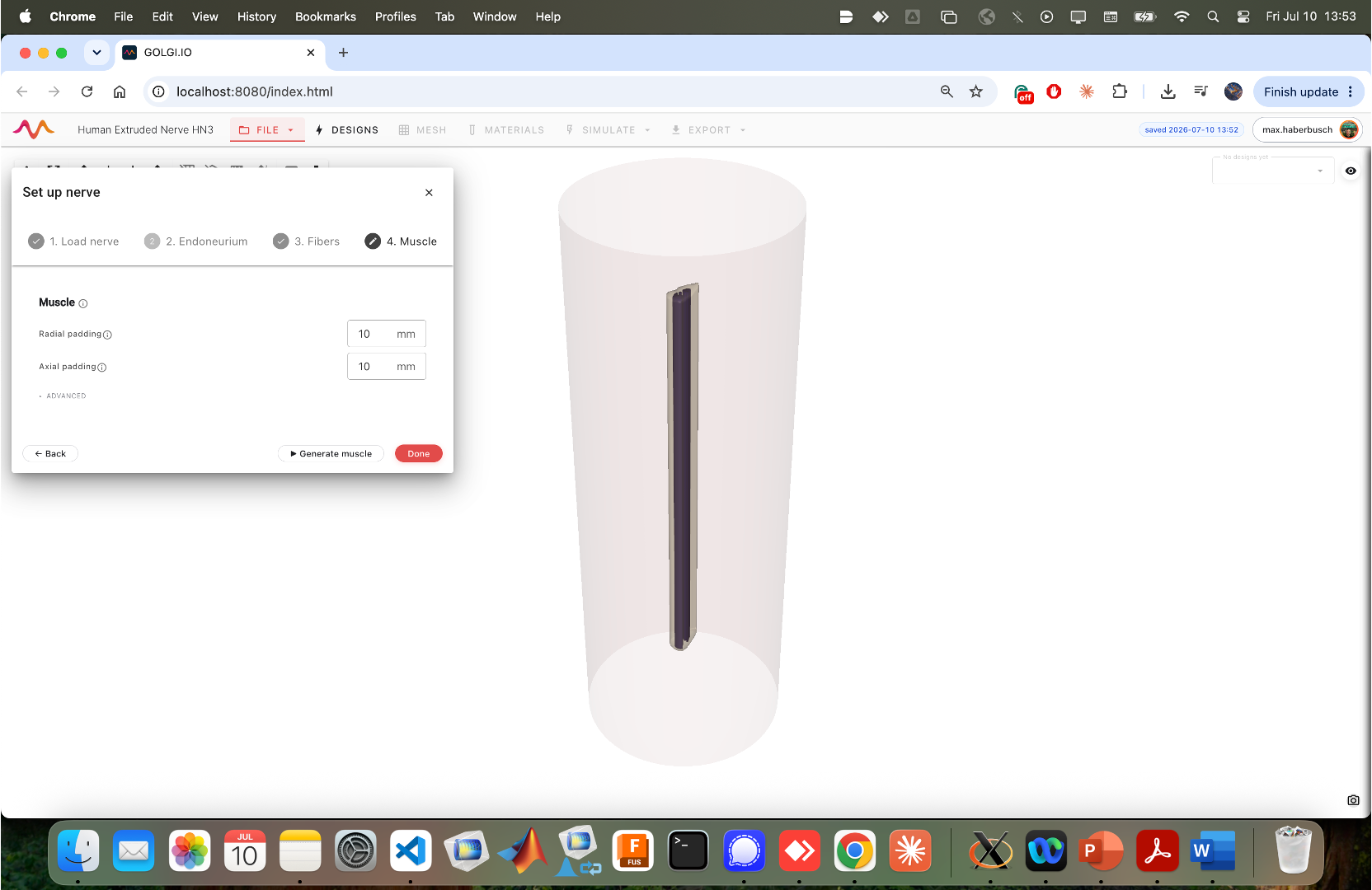
The nerve is now embedded in muscle and ready for electrode design; the workspace switches to the DESIGNS stage.

---

6.4 Design the cuff electrode

On the DESIGNS tab, the Cuff designs panel opens on the right. Initially it is empty ("No designs yet — click + Add to place one."). Use + Add to place a cuff, or + Sweep to create a parametric family of designs.

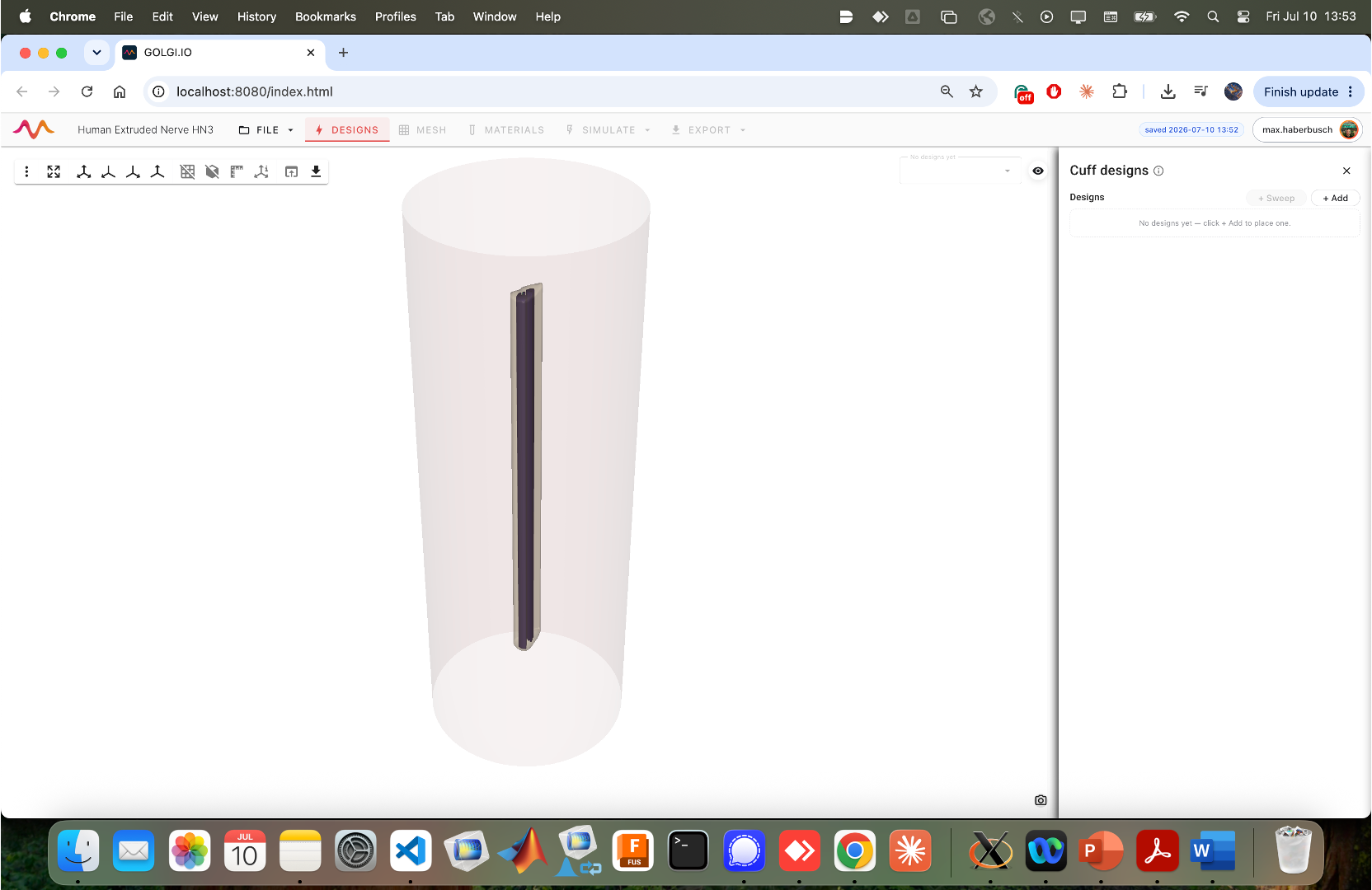
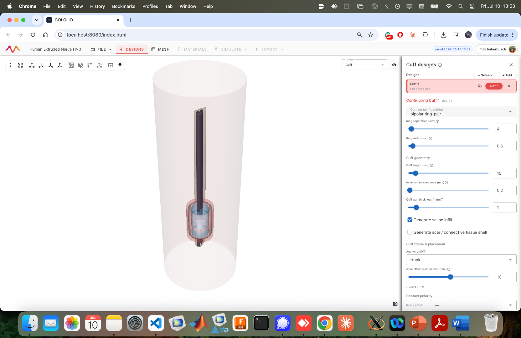
Adding a cuff creates Cuff 1 and opens its configurator. Work through the groups (each has an info tooltip and a slider + numeric field):

• Contact configuration. The electrode montage, e.g. bipolar ring-pair.
• Ring geometry. Ring separation (mm) and Ring width (mm).
• Cuff geometry. Cuff length (mm), Inner radius clearance (mm) (gap between the nerve and the cuff wall) and Cuff wall thickness (mm).
• Generate saline infill — fill the cuff–nerve gap with saline (recommended; it is the conductive medium inside the cuff).
• Generate scar / connective tissue shell — optionally wrap the cuff in an encapsulation layer.

Scroll down for placement and polarity:

• Cuff frame & placement. Anchor end (e.g. trunk) and Axial offset from anchor (mm) position the cuff along the nerve.
• Contact polarity (Advanced). Assign each contact as Anode or Cathode, optionally starting from a Quick preset (e.g. equal-split cathode/anode). Save named Configurations with + Save current so you can compare montages later; the default is called Default.

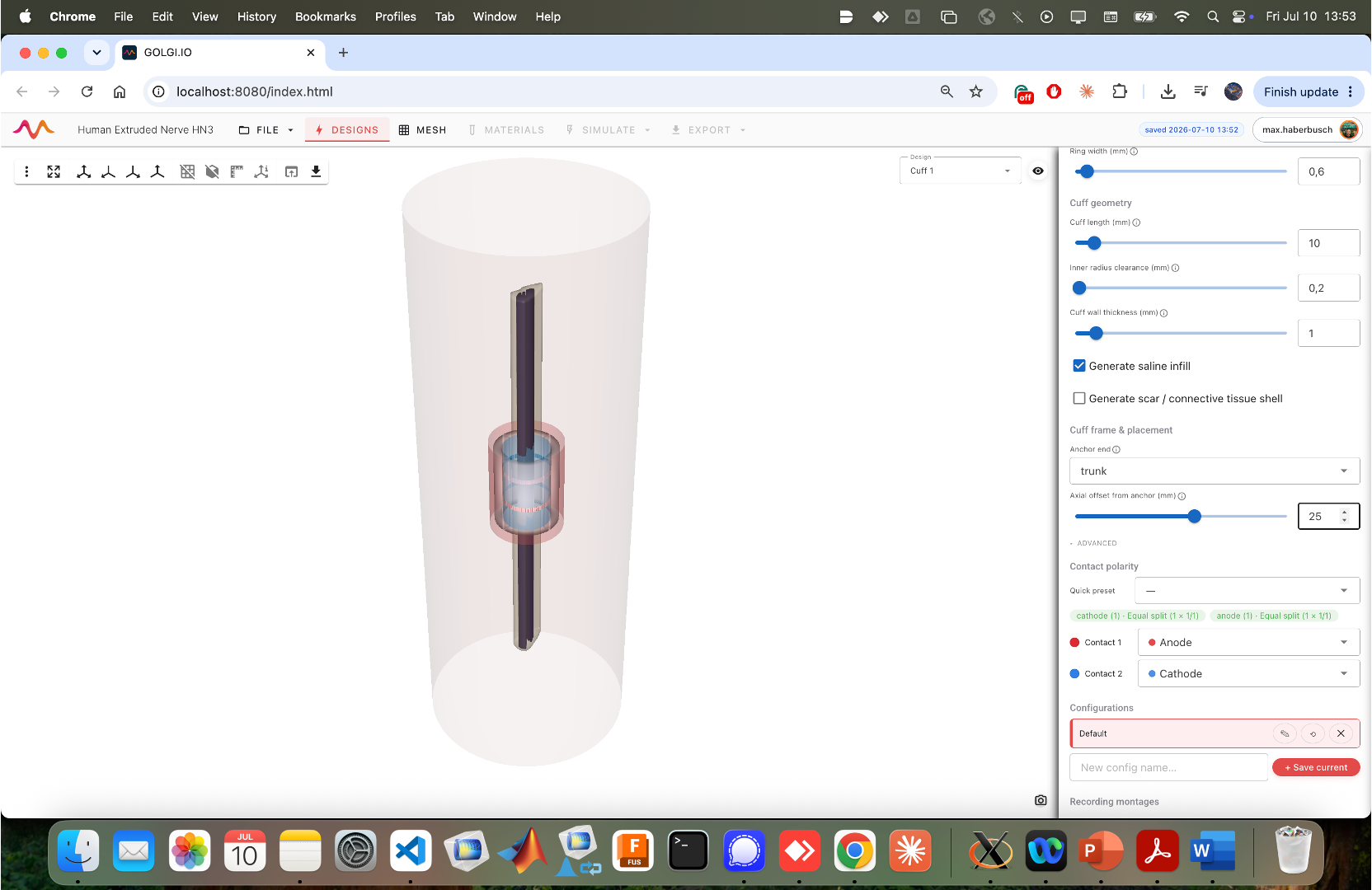
The 3-D viewport updates live as you edit — you can see the ring contacts, the saline infill, and the cuff shell wrap around the nerve. The full range of contact types (tripolar, ring-arrays, helical LivaNova-style, LIFE/TIME, ASCENT/DUKE presets) and the interactive cuff designer are covered on Electrodes & Cuff Designer.

---

6.5 Build the finite-element mesh

Switch to the MESH tab to open the Mesh build panel. At the top, a toggle selects the mesher — gmsh (conformal, robust; it auto-falls back to TetGen for true-3-D nerves or on error).

Set target element sizes (in µm) for each region:

• Tissue region mesh sizes — Endoneurium (e.g. 200), Epineurium (250), Muscle (3000), Scar / connective tissue (150).
• Cuff region mesh sizes — Saline (300), Silicone (300), Contacts (100). Contacts are meshed finest because the field gradients are steepest there.

Under Designs to mesh, pick which cuff design(s) to build meshes for (an empty list just meshes the active design). The panel tells you how many meshes it will build.

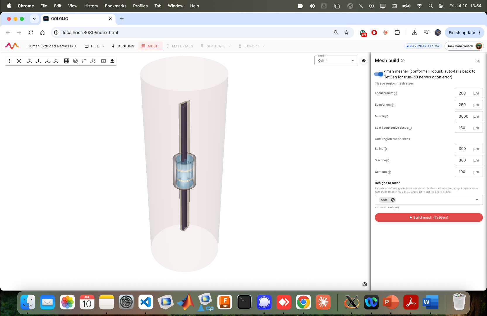
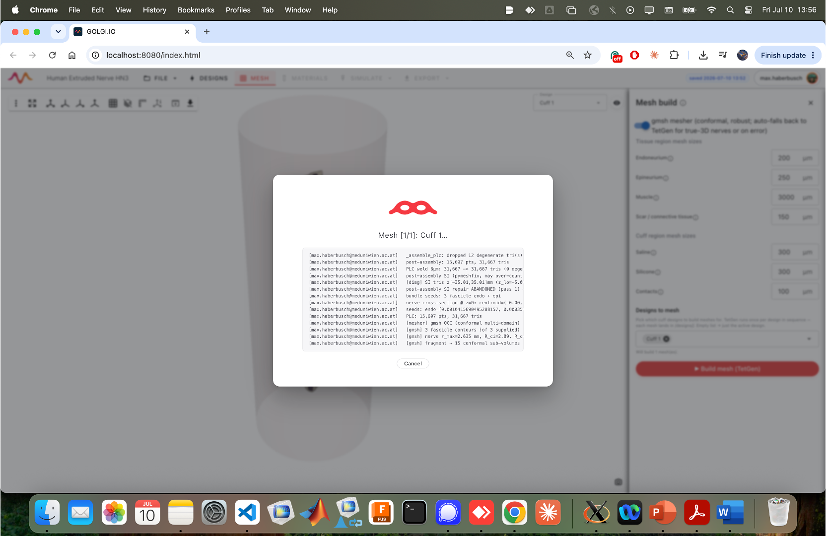
Click ► Build mesh (TetGen). A progress dialog streams the mesher log — surface assembly, PLC welding, per-fascicle contour handling, conformal sub-volume creation, and so on.

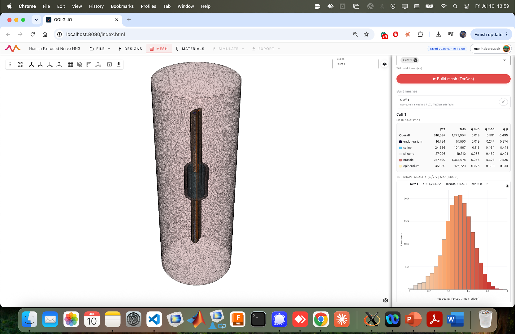
When it finishes, the built mesh appears under Built meshes (e.g. Cuff 1 — nerve.mesh + cached PLC / TetGen artefacts), and a Mesh statistics table reports point and tetrahedron counts and shape quality (q min, q med, q µ) overall and per region (endoneurium, saline, silicone, muscle, epineurium). A Tet shape-quality histogram visualizes the distribution — a peak well away from zero indicates a healthy mesh. See Meshing for the mesher internals and tuning.

---

6.6 Assign material conductivities

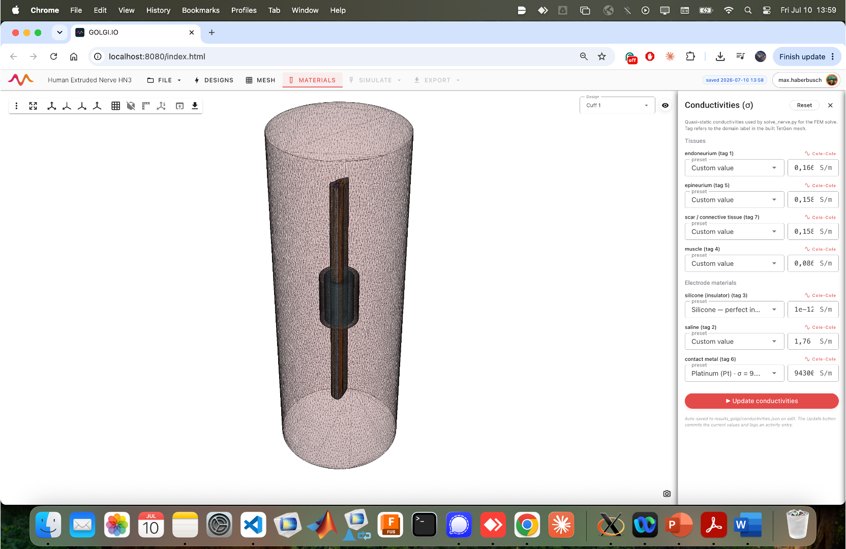
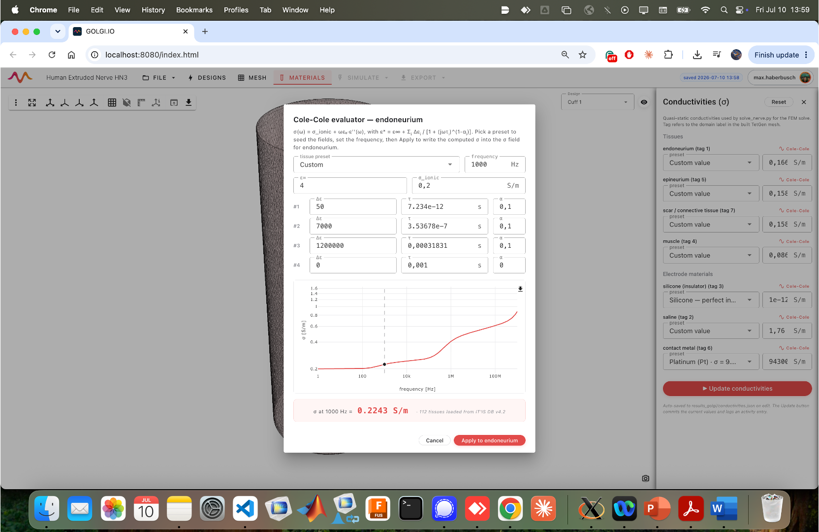
On the MATERIALS tab, the Conductivities (σ) panel lists every meshed region and the quasi-static conductivity used by the field solver. Each row shows the domain tag (matching the built mesh), a preset dropdown, and an editable value in S/m:

• Tissues — endoneurium (tag 1), epineurium (tag 5), scar / connective tissue (tag 7), muscle (tag 4).
• Electrode materials — silicone (insulator) (tag 3, essentially non-conductive, ~1e-12 S/m), saline (tag 2), contact metal (tag 6, e.g. Platinum).

Edit a value directly, or choose a preset. Click ► Update conductivities to commit the values (this also logs an activity entry). Values auto-save on edit.

For frequency-dependent tissue, click the Cole-Cole link on a row to open the Cole-Cole evaluator. This computes an effective conductivity from a four-term Cole-Cole dispersion model. Pick a tissue preset (the database is the IT'IS tissue-properties database), set the Frequency (Hz), and the evaluator plots σ across frequency and reports σ at the chosen frequency (e.g. σ at 1000 Hz = 0.2243 S/m). Click Apply to to write the computed value back into the conductivity table. The tissue models and anisotropy are detailed on Conductivity & Tissue Properties.

The model is now fully specified — geometry, mesh and materials. Chapter 4 solves the field and runs the fibers.

---

← Projects & Workspace · Simulate & Export →