Tutorial Simulate and Export

Tutorial · Simulate & Export

GUI Tutorial · Chapter 4 of 4 — with a meshed, material-assigned model from Build a Model, solve the extracellular field, run single-fiber and population activation, and export the results.

---

6.7 Simulate the extracellular field (FEM)

Open SIMULATE → Extracellular field (FEM). The right panel configures the solve; the left/center panels hold the result plots (initially empty).

• Stimulus. Set the Cathodic stimulation current (mA) (e.g. 1).
• Solver preset. Choose a preset such as Balanced (a compromise between speed and accuracy; presets tune the iterative solver and core count).
• Configs to solve. Pick which saved cuff polarity configurations to solve (e.g. Cuff 1 · Default); All / None select every or no config. Each solve reuses the parent design's mesh, so there is no remeshing.
• Outputs. Tick Compute electrode access impedance (Z_access) on each solve to also report per-contact and per-pair access impedance.

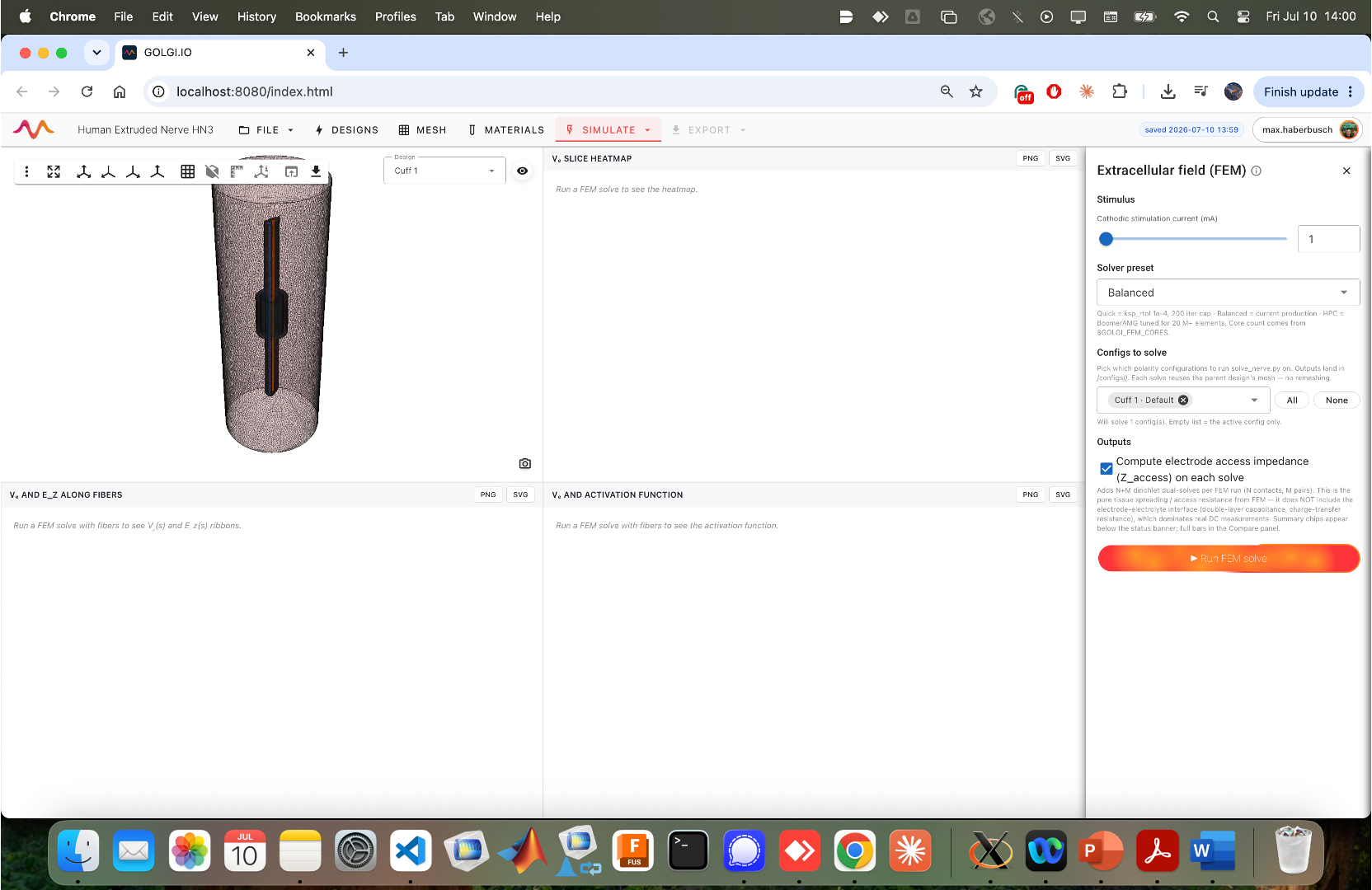
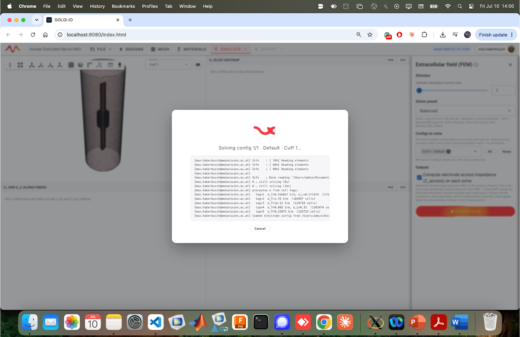
Click ► Run FEM solve. A dialog streams the solver log — reading elements, assigning per-tag conductivities, and solving the linear system.

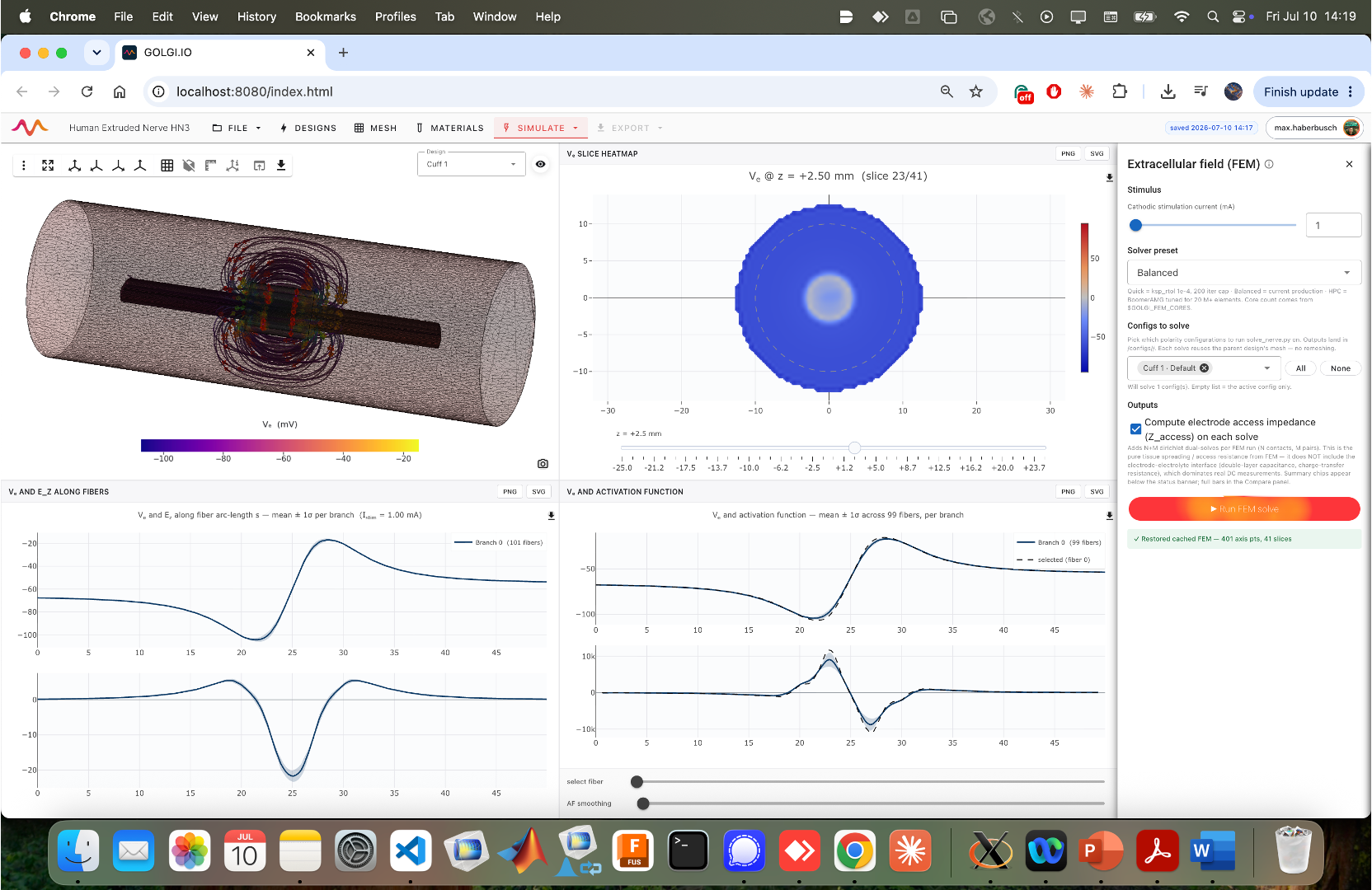
When the solve completes, three linked figures populate:

• Vₑ slice heatmap — the extracellular potential on a cross-section at a chosen axial position (scrub the z slider).
• Vₑ and Eᵤ,z along fibers — potential and its along-fiber gradient versus arc length, shown as mean ± 1σ ribbons per branch.
• Vₑ and activation function — the potential and the activation function (the second spatial derivative ∂²Vₑ/∂z², the classic predictor of where a fiber depolarizes), again per branch.

Each figure can be exported as PNG or SVG. The solver, its presets, the perineurium contact-impedance model and access impedance are all covered on Finite-Element Solver.

---

6.8 Simulate a single fiber

With a solved field in hand, open the SIMULATE menu to reach the fiber solvers: Single fiber, Fiber population, Sweep (recruitment / threshold) and Compare configurations.

Choose Single fiber to open the Single fiber — playground. Pick one or more trajectories to test (e.g. a few fibers from each branch). Then design the stimulus and the fiber model:

• Pulse design. Pulse Type (e.g. monophasic), Polarity (cathodic), Onset (ms), Amplitude (mA) and Pulse Width (µs). The designed waveform is plotted alongside.
• Fiber model. Backend (e.g. pyfibers), Fiber Model (e.g. MRG_INTERPOLATION, a double-cable myelinated-axon model), and the axon Diameter (µm).
• Simulation Duration (ms).

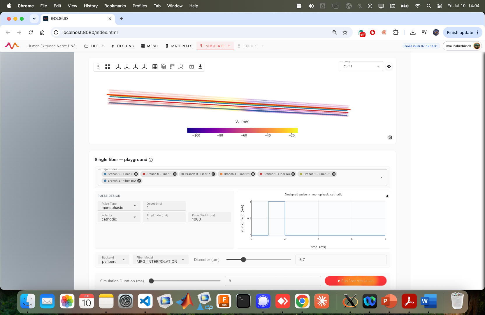
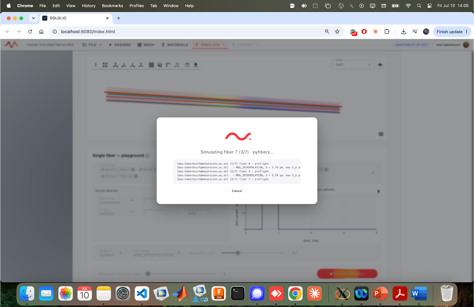
Click ► Run fiber simulation. Each selected fiber is solved in turn (a "Simulating fiber…" dialog reports progress and per-fiber preflight info).

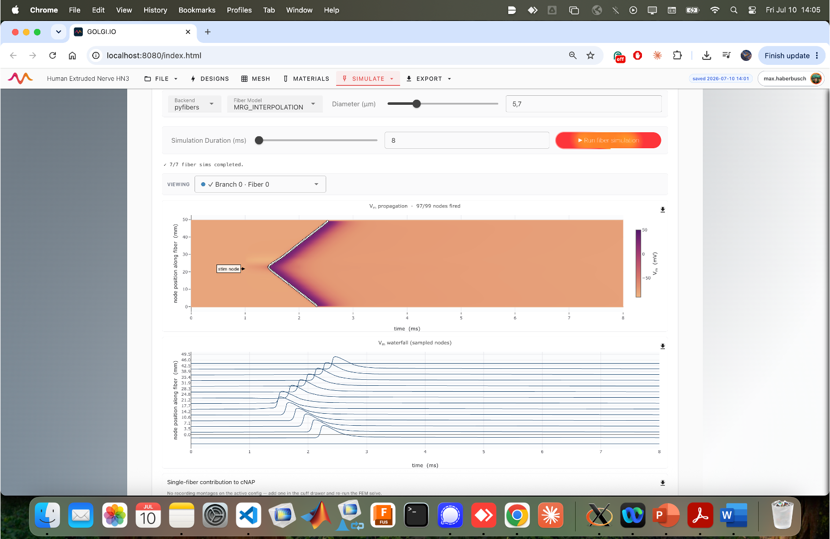
Results appear below. Choose which fiber to inspect with the Viewing dropdown. The key plots are:

• Vₘ propagation — a space–time heatmap of transmembrane voltage along the fiber; the header reports how many nodes fired (e.g. 97/99 nodes fired), and the "stim node" marker shows the point nearest the cathode. A clean V-shaped wavefront that reaches both ends indicates a propagating action potential.
• Vₘ waterfall — the same data as stacked traces at sampled nodes.
• Single-fiber contribution to cNAP — the fiber's contribution to the compound nerve action potential (populated when recording montages are defined on the active cuff configuration; see Recording & CNAP).

The fiber models (MRG variants, SUNDT, AxonML) and the thresholding path are described on Fiber Models & Activation.

---

6.9 Simulate a fiber population

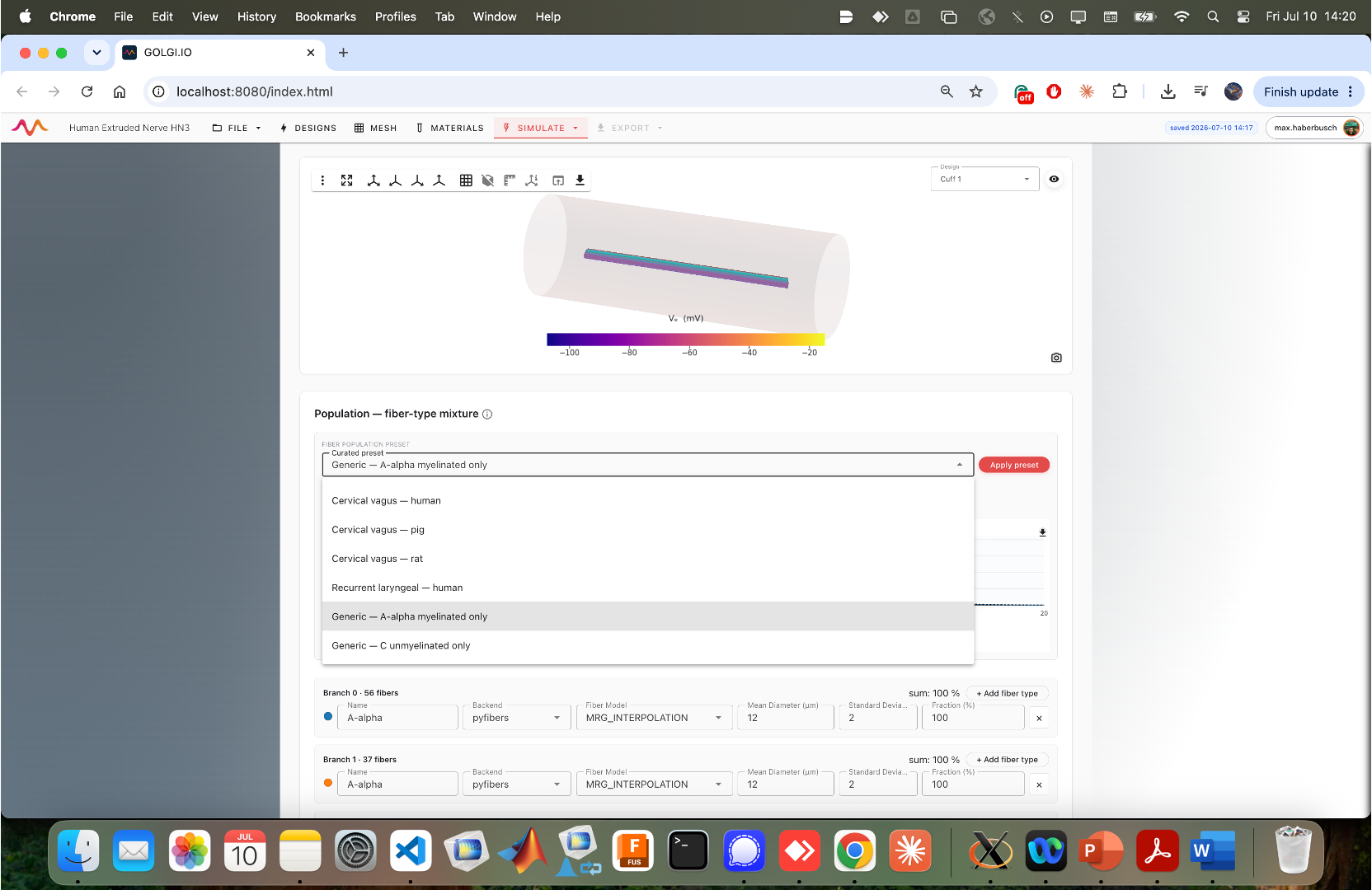
Choose SIMULATE → Fiber population to open the Population — fiber-type mixture builder, which assigns realistic distributions of fiber types to each branch.

Start from a Fiber population preset. The dropdown offers curated mixtures such as Cervical vagus — human / pig / rat, Recurrent laryngeal — human, and generic options (A-alpha myelinated only, C unmyelinated only).

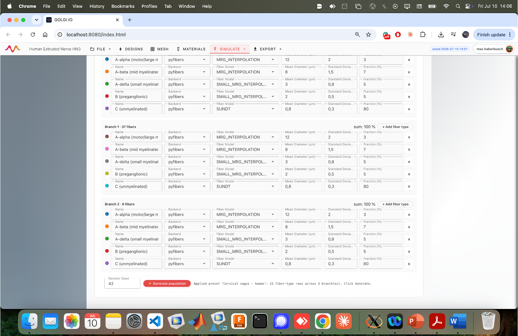
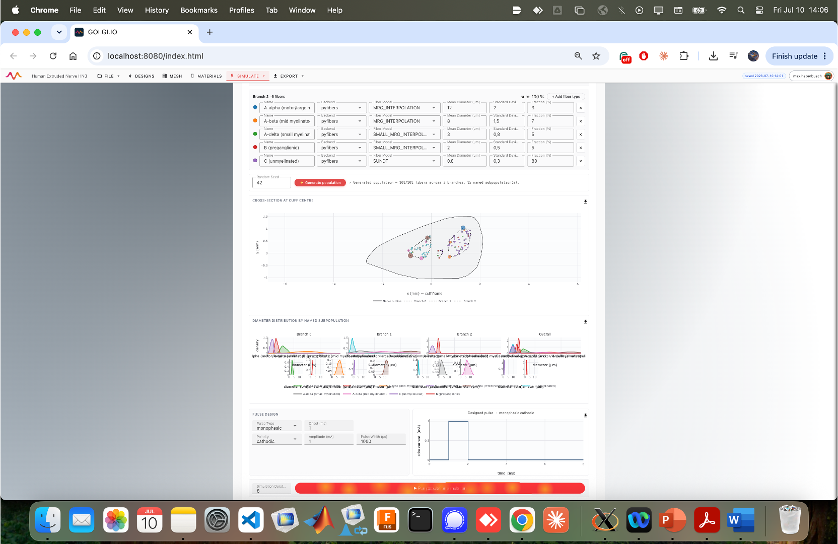
Applying a preset (here Cervical vagus — human) fills each branch with named subpopulations. Every row defines a fiber type: Name (e.g. A-alpha (motor/large myelinated), A-beta, A-delta, B (preganglionic), C (unmyelinated)), Backend, Fiber Model (myelinated types use MRG variants; unmyelinated C fibers use SUNDT), Mean Diameter (µm), Standard Deviation, and Fraction (%). The fractions per branch must sum to 100 %. Use + Add fiber type to add rows and the ✕ to remove them. Set a Random Seed for reproducibility.

Click ► Generate population. golgi samples concrete fibers from the mixture and reports the result (e.g. Generated population.run — 101/101 fibers across 3 branches). Two diagnostics appear:

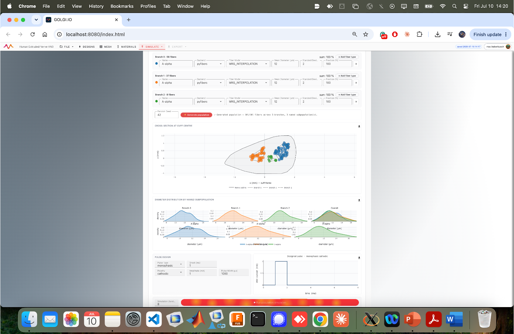
• Cross-section at cuff centre — a scatter of each sampled fiber's position within the nerve outline, colored by branch.
• Diameter distribution by named subpopulation — per-branch and overall diameter histograms/KDEs.

Below them sits the same Pulse design block as the single-fiber tool.

The screenshots also show a simpler Generic — A-alpha myelinated only population (one fiber type per branch), which is handy for a quick, clean test before running a full multi-type mixture.

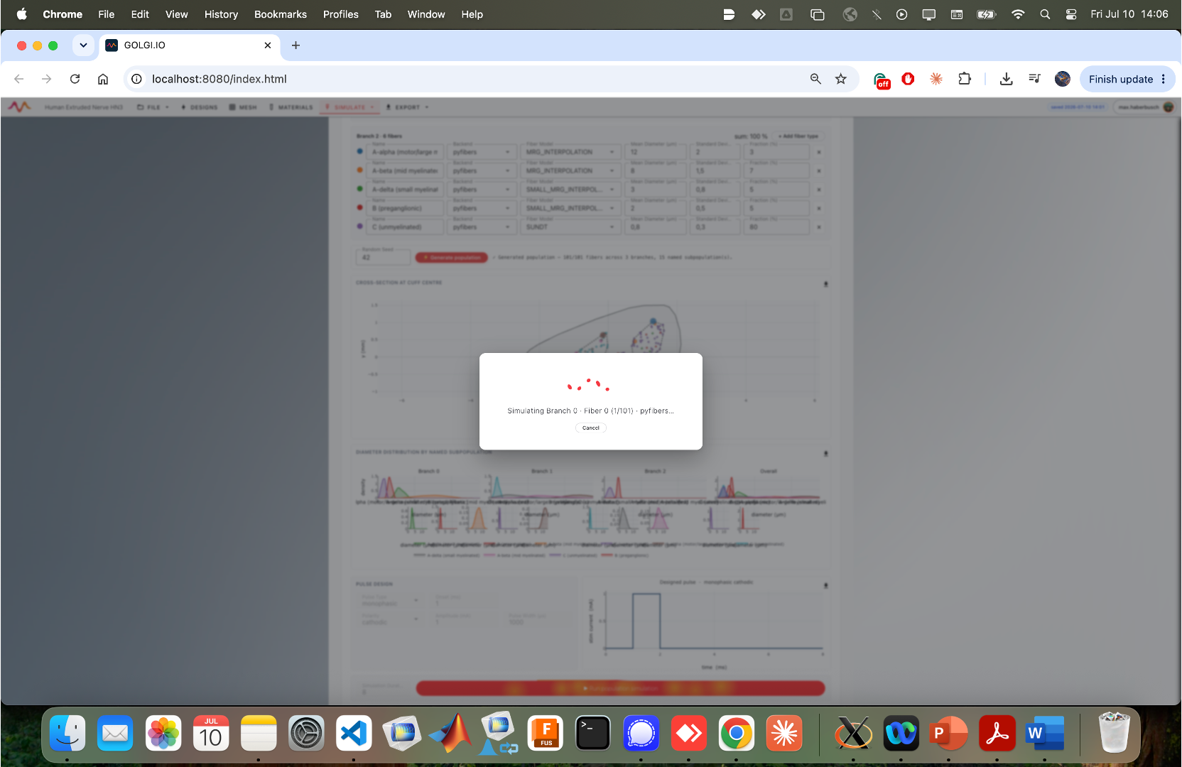
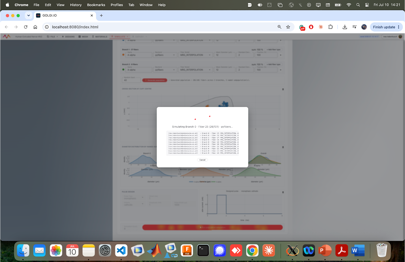
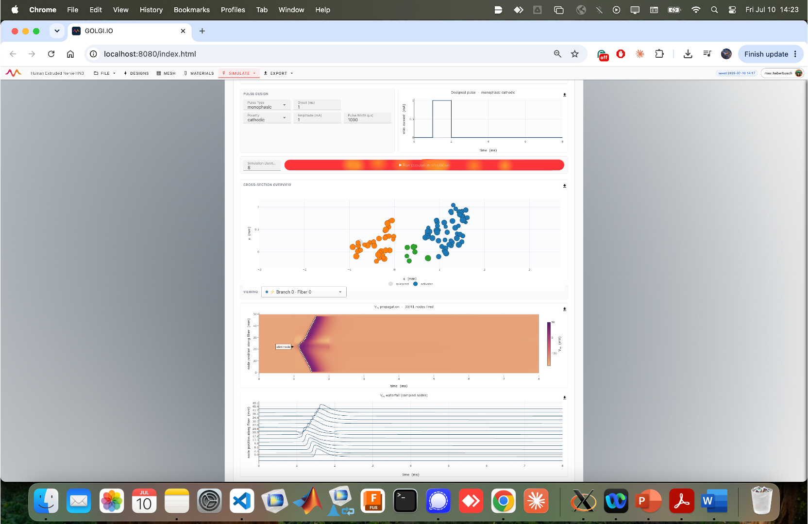
Click ► Run population simulation. Every fiber is solved in turn with a progress dialog ("Simulating Branch 0 · Fiber n/101…").

When the run finishes, the results summarize recruitment across the whole nerve:

• Cross-section overview — the fiber scatter, now colored by outcome (activated vs silent), so you can see which region of the fascicle the cuff recruits at the chosen amplitude.
• Vₘ propagation / waterfall — inspect any individual fiber via the Viewing dropdown, exactly as in the single-fiber tool (e.g. 29/99 nodes fired for a partially activated fiber).

For dose–response behaviour, use SIMULATE → Sweep (recruitment / threshold) to vary the stimulus amplitude and produce recruitment curves and per-fiber activation thresholds. Compare configurations contrasts the outcomes of different saved cuff polarity configurations. Both are covered on Recruitment Sweeps & Selectivity.

---

6.10 Export figures and generate a report

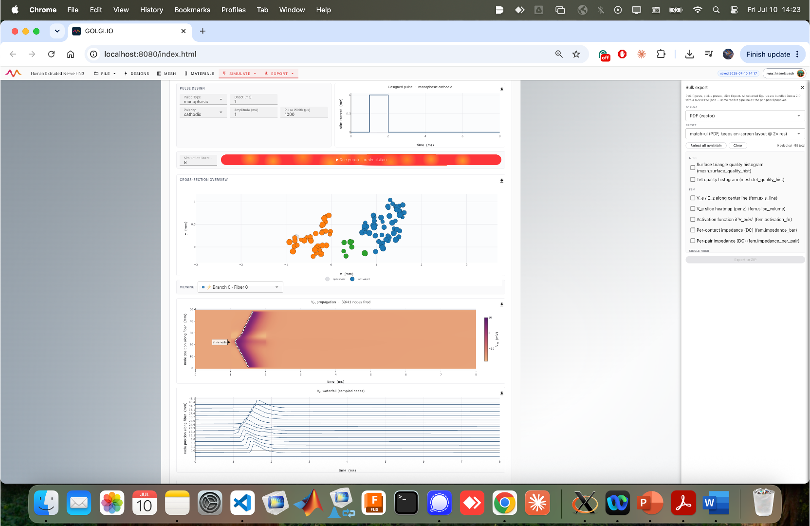
Open the EXPORT tab for the Bulk export panel. Choose a Format — PDF (vector) or match-ui (a PDF that preserves the on-screen layout at 2× resolution) — then tick the figures to include. They are grouped by stage:

• Mesh — surface-triangle quality histogram, tet-quality histogram.
• FEM — Vₑ / Eᵤ,z along centerline, Vₑ slice heatmap (per z), activation function ∂²Vₑ/∂z², per-contact impedance, per-pair impedance.
• Single-fiber and population figures.

Use Select all available / Clear to toggle everything, then export to a ZIP.

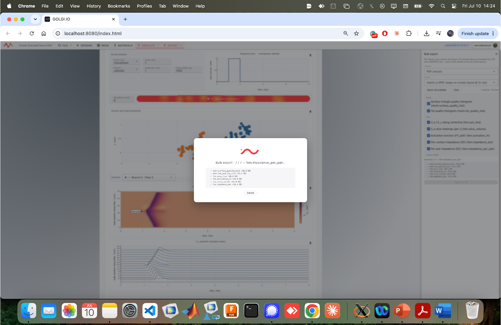
A progress dialog lists each figure as it is rendered and written.

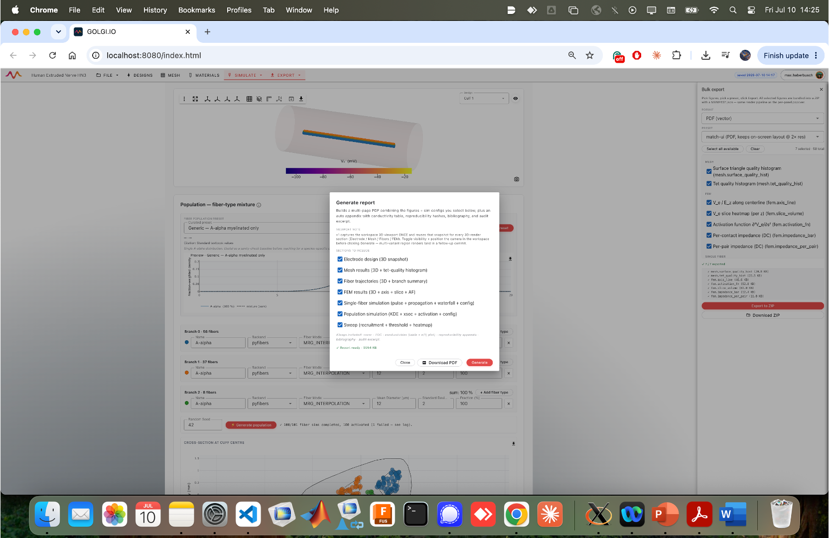
To produce a single narrative document instead, use Generate report. It builds a multi-page PDF that combines the figures with the configs you select, plus an auto-appendix (conductivity table, reproducibility hashes, bibliography, and an audit excerpt). Tick the Sections to include:

• Electrode design (3D snapshot)
• Mesh results (3D + tet-quality histogram)
• Fiber trajectories (3D + branch summary)
• FEM results (3D + axis + slice + AF)
• Single-fiber simulation (pulse + propagation + waterfall + config)
• Population simulation (KDE + cross-section + activation + config)
• Sweep (recruitment + threshold + heatmap)

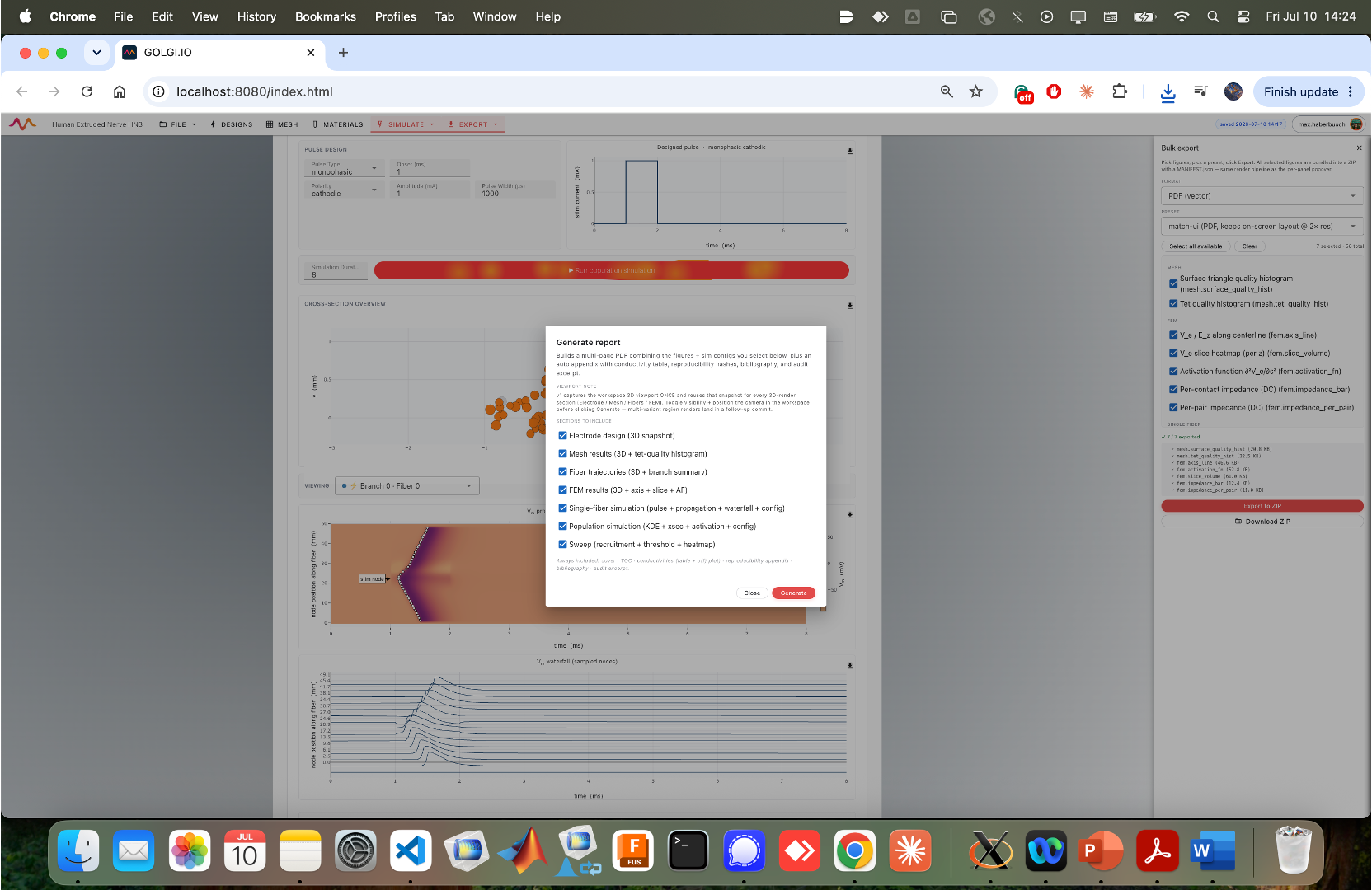
Click Generate. golgi re-renders 3-D snapshots for each requested section and embeds every figure ("Generating report — rendering 3D variants + embedding figures…"). Position the 3-D viewport camera first — the report captures it once. See Figures & Reports for the export formats and report layout.

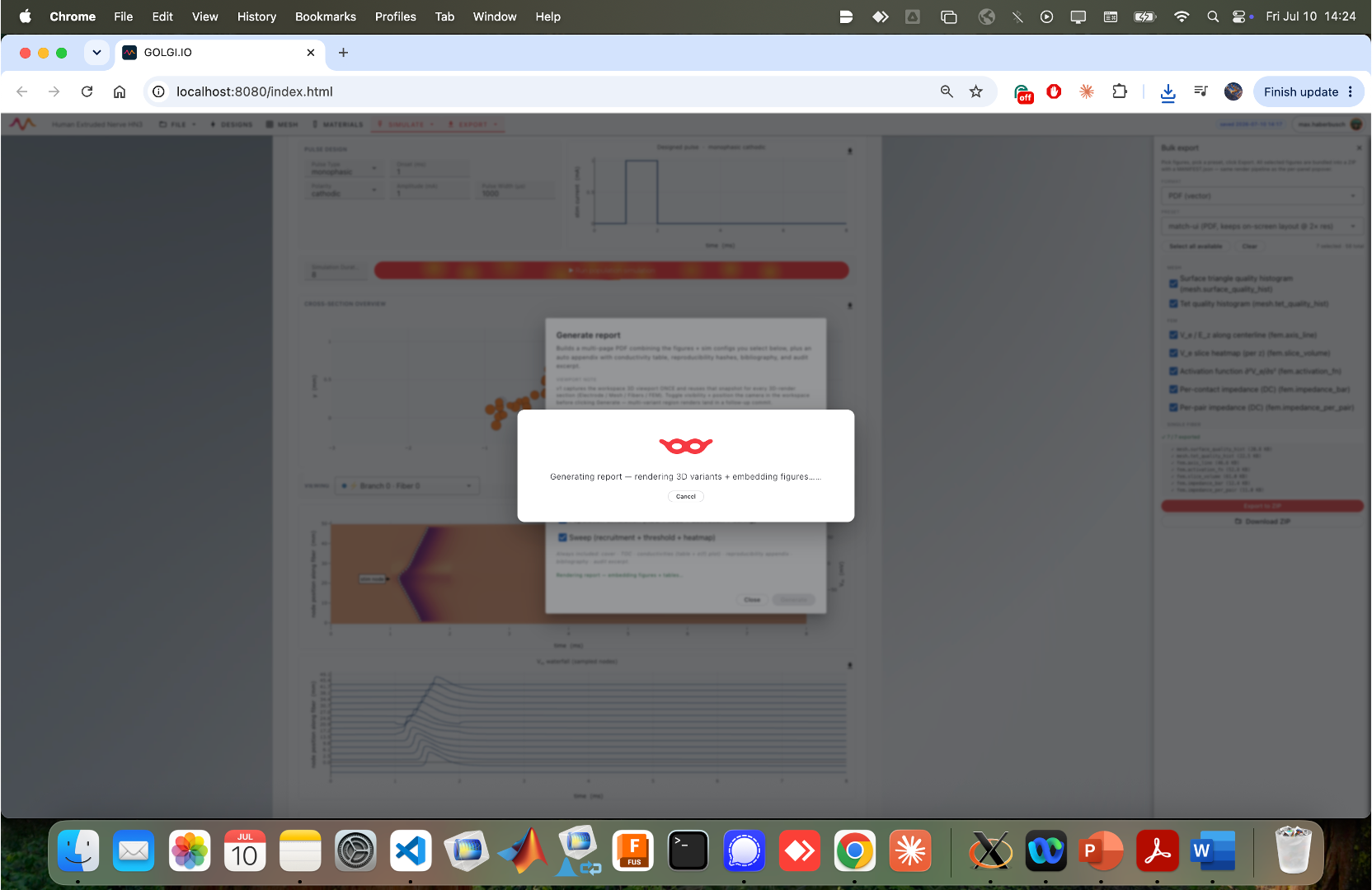
When it is done, the dialog reports the finished size and offers Download PDF (and you can Generate again after changing sections).

---

Exporting and importing study bundles

Beyond exporting individual figures, golgi can archive an entire study for sharing or reproduction. There are two equivalent entry points:

• From the dashboard, open a project card and click Export study (see Projects & Workspace).
• From inside the workspace, use FILE → Export study….

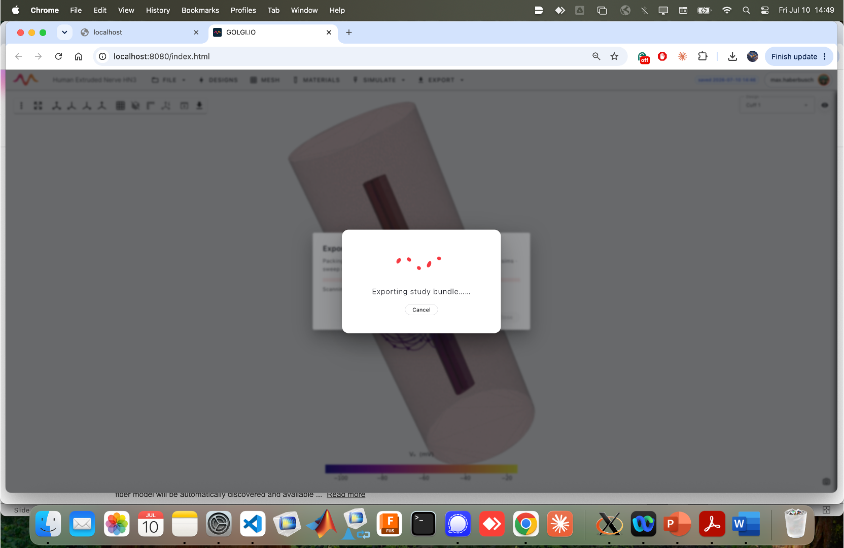
Either way, golgi packs every project file — configs, mesh, FEM outputs, fibers, simulations, sweep results and an audit excerpt — into one self-contained .zip. A progress dialog appears while packing.

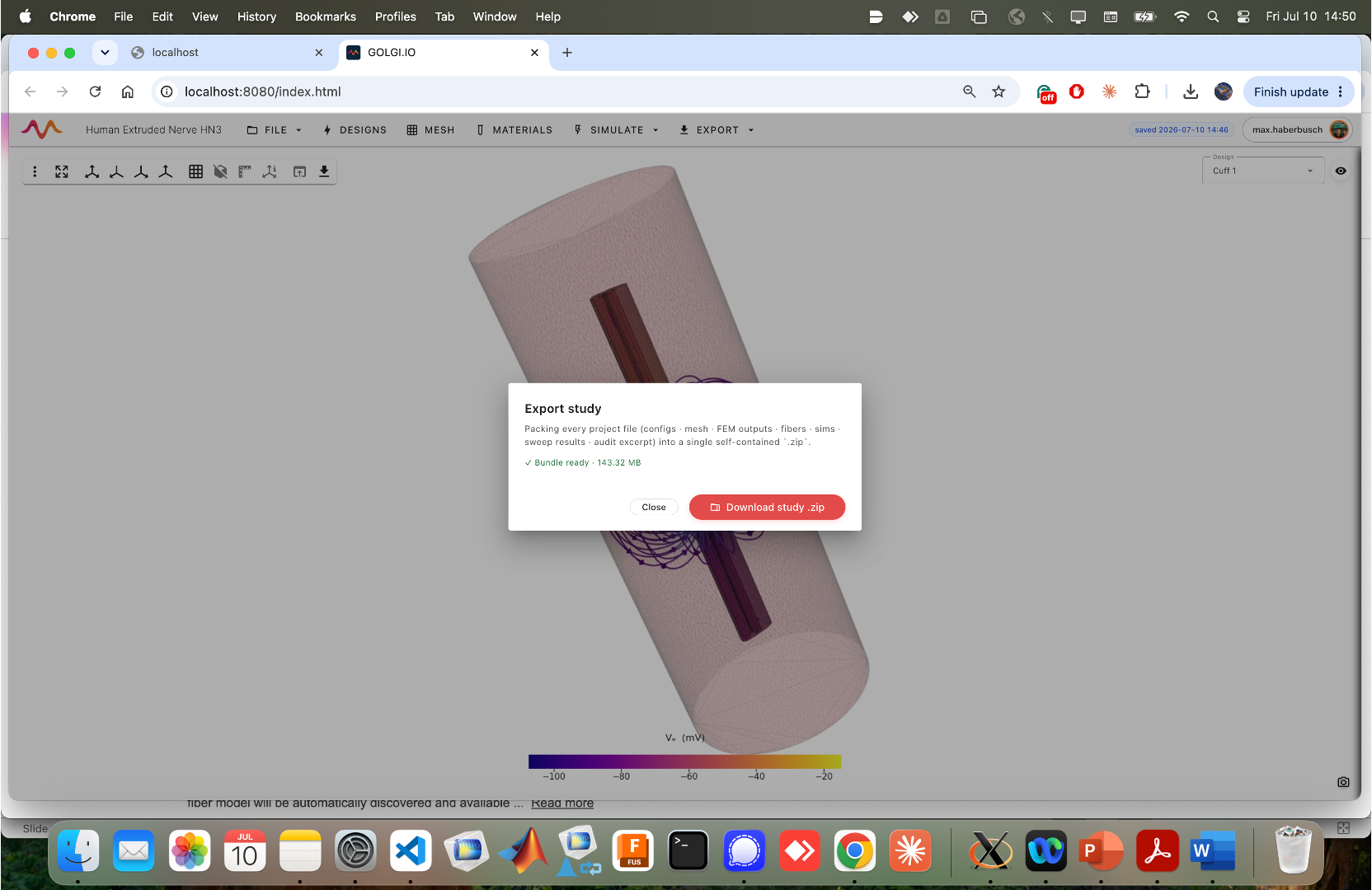
When packing completes, the popover shows "Bundle ready" with the archive size and a Download study .zip button. (Bundle size scales with how much of the pipeline has been computed and cached.)

To reload a shared study, use FILE → Import study… and select a .zip produced by Export study. Because the bundle carries the cached results and the audit log, the imported project restores to the same state — a reviewer can open it and reproduce every figure without rerunning the solvers. The bundle format, integrity hashing and replay verification are covered on Reproducible Study Bundles.

---

That completes the tutorial — you have taken a nerve from a raw µCT image all the way to a whole-population activation report and a shareable, reproducible study bundle. From here:

• Script the same pipeline → Python API · Command-Line Interface
• Run at scale → Headless / HPC
• Reproduce the paper figures → Reproducing the Paper
• Look up a term → Glossary

---

← Build a Model · Tutorial overview