Warp drives

Warp drives

extensions/warp/ ports WarpFactory, a toolkit that analyzes warp drive spacetimes in general relativity. It samples a metric on a grid and finds the stress-energy tensor by the Einstein equations. It then checks the energy conditions and finds the expansion, shear and vorticity. The port runs on the CPU in Float64, on every core.

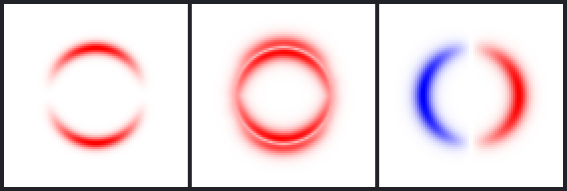
Rendered by examples/warp_drive.mojo. The bubble moves along x at half the speed of light. The panels cut the plane z = 0. From the left, they show the energy density, the null energy condition and the expansion. Red is negative, blue is positive and white is zero.

The port follows WarpFactory at commit 03b10cb, dated 2024-05-23. Its method is in Helmerich et al. (2024). The port also adds exact derivatives, more metrics, energy totals, spherical and cylindrical grids, and geodesics. To learn the steps one at a time, follow Tutorial: Analyze a warp drive.

Modules

Module	What it gives	WarpFactory
kinds	Axis, TensorIndex, EnergyCondition, DifferenceOrder, Frame and CoordinateSystem	The strings "covariant", "Null", "fourth" and others
quantities	EnergyDensity64, SPEED_OF_LIGHT, GRAVITATIONAL_CONSTANT and fraction_of_light	Units/
grid	SpacetimeGrid and SpacetimeCenter	gridSize, gridScaling and worldCenter
tensor	TensorField, Metric, change_index and trace	The tensor struct, changeTensorIndex, getTrace, c4Inv
three_plus_one	ThreePlusOne and decompose	threePlusOneBuilder and threePlusOneDecomposer
metrics	Minkowski, Alcubierre, Lentz, Van Den Broeck, modified time and Schwarzschild	Metrics/
natario	A drive with zero expansion	None
krasnikov	The Krasnikov tube	None
fell_heisenberg	The positive-energy soliton of Fell and Heisenberg	None
warp_shell	The warp shell, shells from any profiles, and an accelerating shell	metricGet_WarpShellComoving
curvilinear	Metrics on spherical and cylindrical grids	None
derivatives	derivative, second_derivative and Stencil	takeFiniteDifference1 and 2
solver	stress_energy and curvature	getEnergyTensor, ricciT, ricciS, einT, einE
gpu	gpu_stress_energy, gpu_curvature and warp_gpu_available	getEnergyTensor with its GPU option
jet, analytic	Exact derivatives of closed-form metrics, and the exact solver	None
frame	to_eulerian and eulerian_transform	doFrameTransfer and getEulerianTransformationMatrix
conditions	energy_condition, energy_condition_samples and the sampled directions	getEnergyConditions and generateUniformField
scalars	metric_scalars	getScalars
totals	energy_totals and violation_total	None
flow	momentum_flow_lines	getMomentumFlowLines
geodesics	trace_geodesic, proper_time and passenger_view	None
evaluation	evaluate_metric	evalMetric
plot	slice_plane, red_blue, draw_plane and draw_plane_range	getSliceData and redblue

Analyze a metric

Make a grid, build a metric on it, and call evaluate_metric. The result holds the stress-energy tensor, the four energy conditions and the three scalars.

On the GPU

gpu_stress_energy and gpu_curvature in extensions/warp/gpu.mojo solve the Einstein equations on a GPU through MAX. One thread solves one point. The kernel calls solve_point, the function that the CPU tasks call, so both take the same differences and the same Ricci tensor. The results agree with the CPU's to 1e-12 of each point's largest component. They are not equal bit for bit, because a GPU compiler can fuse a multiply and an add that the CPU rounds twice.

The solver uses 64-bit floats. A Metal GPU has no 64-bit floats, so on Apple silicon the two functions refuse to run, and warp_gpu_available returns False. Use stress_energy there.

from extensions.warp.evaluation import evaluate_metric
from extensions.warp.grid import SpacetimeGrid
from extensions.warp.metrics import alcubierre_comoving
from extensions.warp.quantities import fraction_of_light
from units.si import Duration64, InverseLength64, Length64

var grid = SpacetimeGrid.uniform(
    1, 20, 20, 20, Duration64(1.0), Length64(1.0)
)
var metric = alcubierre_comoving(
    grid,
    grid.center(),
    fraction_of_light(0.5),
    Length64(5.0),
    InverseLength64(0.5),
)
var result = evaluate_metric(metric)
print(result.null.worst().value)         # the most negative value, J/m^3
print(result.null.violations())          # points that violate it
print(result.eulerian.tensor.get(0, 0, grid.index(0, 10, 13, 10)))

Each step is also a function of its own. Call stress_energy for the tensor and to_eulerian to move it into the Eulerian frame. Call energy_condition for one condition and metric_scalars for the scalars.

The solver, the exact solver, the energy conditions and the passenger view split the points among one task for each logical core. Pass threads to choose the count. Each point is computed alone, so every count gives the same values, bit for bit.

The grid

A SpacetimeGrid has a count of points and a step along t, x, y and z. The time step is a Duration64, and the space steps are Length64 values. The grid holds at most 1048576 points. A tensor of that size takes 128 MiB.

The time coordinate is x⁰ = c t. So every coordinate is a length, the metric is dimensionless, and every stress-energy component is in J/m³. WarpFactory gets the same result when it divides each time derivative by c.

A SpacetimeCenter is the place of the origin. Point i along an axis sits at (i + 1) times the step, minus the center. Indexes count from 0, but this keeps the places of WarpFactory, which counts from 1. grid.center() puts the origin in the middle of the grid, as the WarpFactory examples do.

The derivatives need points on both sides. The fourth-order stencils need 5 points along an axis, and the second-order stencils need 3. An axis with fewer points has no derivative. So a grid with one time slice is static.

Spherical and cylindrical grids

SpacetimeGrid.spherical makes a grid in t, r, θ and φ. SpacetimeGrid.cylindrical makes one in t, ρ, φ and z. Point i along an axis sits at the start plus i steps. A spherical shell needs far fewer points in these coordinates, because its features lie along r.

The grid must start away from the axis and the poles, where the coordinates are singular. If the φ points cover a whole turn, the stencils wrap around the circle.

The solver, the Eulerian frame, the energy conditions, the scalars and the totals read only the metric and its derivatives. So they work in any coordinates. The builders in curvilinear give metrics on these grids.

Function	Grid	Metric
minkowski_curvilinear	Spherical or cylindrical	Flat space
schwarzschild_spherical	Spherical	A black hole in Schwarzschild coordinates
warp_shell_spherical	Spherical	The warp shell, with its polar axis along the direction of travel
alcubierre_cylindrical	Cylindrical	The comoving Alcubierre bubble, moving along z

In curvilinear coordinates the components in the coordinate frame have mixed units: g_θθ = r² is in square meters. The components in the Eulerian frame are all in J/m³. The other builders, the flow lines and the closed-form metrics need a Cartesian grid, and refuse any other.

Build a metric

Each metric function takes the grid and the center. Then it takes the metric's own parameters, each with its unit.

Function	Parameters	Time slices
minkowski	None	Any
alcubierre, alcubierre_comoving	Speed, radius R, steepness σ	5 or more, or 1
lentz, lentz_comoving	Speed, size of one region	5 or more, or 1
van_den_broeck, van_den_broeck_comoving	Speed, R₁, σ₁, R₂, σ₂, expansion A	5 or more, or 1
modified_time, modified_time_comoving	Speed, R, σ, lapse factor A	5 or more, or 1
natario, natario_comoving	Speed, R, σ	5 or more, or 1
krasnikov	δ, wall ε, length D, radius ρ_max	5 or more
fell_heisenberg	A FellHeisenbergSoliton: Π, r, V, σ, tilt k, scale L	Any
schwarzschild	Schwarzschild radius	1
warp_shell_comoving	Mass, R₁, R₂, buffer, σ, smoothing, speed, warp	1
shell_from_profile	Radial profiles of g_tt, g_rr and the shift, speed	Any
accelerating_shell	Profiles, start and end speeds, start time, duration	5 or more

A _comoving function gives the metric in the frame that moves with the drive. It needs one time slice. The other functions move the drive across the time slices.

To build a metric of your own, start from ThreePlusOne(grid). Set the lapse, the shift β_i and the spatial metric γ_ij at each point. Then call metric(name). For exact derivatives, write it as an AnalyticMetric instead: see Exact derivatives.

More metrics

The Natário drive moves a bubble without expanding or contracting space. Its flow of space is a curl, so its divergence is zero for any shape. This port derives the shift from that construction. It is not copied from Natário's paper, which this port could not check. The tests show that the expansion is zero to rounding.

The Krasnikov tube is a passage that a ship lays down on its way out. Inside it, the way back is short. The metric is Everett and Roman's four-dimensional tube. The port uses the quintic smooth step 6u⁵ - 15u⁴ + 10u³ for its walls. Inside the tube g_xx is negative, so the Eulerian frame does not exist there, and to_eulerian refuses those points.

shell_from_profile builds a static spherical shell from any radial profiles of g_tt, g_rr and the shift. It is the general form of the warp shell. Bobrick and Martire describe warp drives as shells of this kind.

accelerating_shell changes the speed inside a shell over time, along a smooth step. How to accelerate a physical warp shell is an open question. This metric is a test case, not a solution. The tests show one result. Inside the shell, a shift that changes only with time leaves space flat. So any cost of the change is in the shell.

The soliton of Fell and Heisenberg has positive Eulerian energy. Its shift is the gradient of a potential φ, so its momentum density is zero. Its energy density is (h₁ + h₂ + h₃) c⁴ / (8π G). Here h₁, h₂ and h₃ are the 2 × 2 principal minors of the Hessian of φ. FellHeisenbergSoliton gives φ, the shift and this energy density in closed form, and it is an AnalyticMetric.

The paper's potential has two functions m and n that the paper does not give. The port uses m = 1 / (1 - τ) and n = 1 / (1 + τ). Then φ is zero at the center, as the paper asks.

With τ = 0 the soliton is spherical. Its shift is zero inside the radius r and radial outside, and its energy density is positive everywhere. The tilt k sets τ = tanh(k ẑ / u), which makes m larger than n in +z, as in the paper. The center then has a level shift along z of V √(σπ) erf(r/√σ) k. The paper's values (Π, r, V, σ) = (1/4, 6, 10, 1) with k = 0.071 give 1.26, the paper's superluminal center. The tilted soliton is not proven positive: check its energy density on a grid.

The last product of the paper's equation 13 must read m (n r + u), not m (n r - u). Only then does the shift vanish inside and fall off outside, as the paper says. The tests check the potential against equation 13 with this change. They check the energy density against the exact Einstein equations and the finite-difference solver.

The warp shell

warp_shell_comoving builds the shell of Fuchs et al. (2024). A shell of ordinary matter holds a static spacetime, and a shift inside it moves the inside along x. The function first builds radial profiles of the density, the pressure and the metric. The pressure comes from the Tolman-Oppenheimer-Volkoff equation for a constant density.

The profiles use WarpFactory's 100000 radial samples. samples changes that count. The shell's Schwarzschild radius must be less than 8/9 of the outer radius. A heavier shell has an infinite pressure at its center.

The grid must reach past the outer radius. The samples reach to 1.2 times the distance of the last grid point, and every grid point must be inside that radius.

Exact derivatives

The closed-form metrics are also structs, such as AlcubierreMetric, NatarioMetric and KrasnikovMetric. Each is an AnalyticMetric: it gives g_ab at any place as jets. A Jet carries a value with its exact gradient and Hessian, by forward automatic differentiation.

exact_stress_energy and exact_curvature take the derivatives from the jets, not from a stencil. There is no step, no truncation error and no edge of the grid. A grid of one point is enough, and a moving drive needs no time slices around it.

var bubble = AlcubierreMetric(
    fraction_of_light(0.5), Length64(2.0), InverseLength64(1.5), True
)
var energy = exact_stress_energy(bubble, grid, center)
var metric = sample_metric(bubble, grid, center)
var rho = to_eulerian(energy, metric).tensor.get(0, 0, point)

sample_metric gives the same metric on a grid, from the same formula, for the finite-difference solver. The Lentz soliton has jumps between its regions, so it has a grid form only.

The energy conditions

energy_condition moves the tensor into the Eulerian frame. Then it samples a set of directions at each point, and keeps the most violating value. A negative value violates the condition.

Condition	Directions	Value at a point
Null	count null directions	min T_ab k^a k^b
Weak	count times shells timelike directions	min T_ab V^a V^b
Strong	count times shells timelike directions	min (T_ab - T η_ab / 2) V^a V^b
Dominant	count null directions	-max s(F) √abs(F·F), with F^a = -T^a_b k^b

The defaults are 100 directions and 10 shells, as in WarpFactory. energy_condition_samples also keeps the value of every direction at every point. ConditionMap.violations_only keeps only the negative values, as evaluate_metric does with keep_positive set to False. Why the energy conditions use the Eulerian frame explains the choice of metric.

Totals

energy_totals adds the Eulerian energy density over one time slice, times the proper volume of each cell. It gives the total in joules, its positive part and its negative part. violation_total adds the negative part of an energy condition map the same way.

For a result of the finite-difference solver, pass margin = 2 to leave out the two outer layers of points. There the stencils copy the nearest derivative. A result of the exact solver has no such layers.

Geodesics

trace_geodesic follows a free particle or a ray of light through a closed-form metric, by the fourth-order Runge-Kutta method. The Christoffel symbols are exact. null_velocity makes the tangent of a ray, and proper_time gives the time on a clock that rides along a worldline.

Rendered by examples/warp_view.mojo. passenger_view traces one ray back in time from a passenger for each pixel, until the ray leaves the bubble. There the observer at rest with the stars names the direction of the sky. The left panel is flat space. The others are from the center of a bubble at 1, 3 and 6 times c. The faster the bubble, the more of the sky crowds into the view ahead.

Views

Rendered by examples/warp_surface.mojo. The surface holds the places where the Eulerian energy density of an Alcubierre bubble is below a third of its least value. It is a ring around the direction of travel. The repository's surface-net mesher makes the mesh, and the renderer draws it.

Rendered by examples/warp_bubble.mojo. The bubble crosses the frame at half the speed of light. The left panel is the energy density and the right panel is the momentum density along x. The exact solver finds each frame at one instant. draw_plane_range gives every frame the same colors.

Units

Quantity	Type	Unit
A stress-energy component, an energy condition	EnergyDensity64	J/m³
A total	Energy64	J
The expansion θ	InverseLength64	1/m
The shear σ² and the vorticity ω²	InverseArea64	1/m²
The Ricci scalar	InverseArea64	1/m²
A warp speed	Velocity64	m/s
The flow line step	Compliance64	m³/J
Proper time	Duration64	s

The fields store plain Float64 values in these units. The accessors, such as StressEnergy.component and ConditionMap.at, return the typed quantity.

Differences from WarpFactory

Each difference corrects a WarpFactory result or makes a refusal explicit.

• The null and weak conditions lower the Eulerian tensor with the Minkowski metric. WarpFactory uses the metric of the coordinate frame for these two, and the Minkowski metric for the other two. The Eulerian frame is orthonormal, so its metric is the Minkowski metric. Where g is not η, the null and weak values differ from WarpFactory's.
• change_index moves a tensor between the two mixed index positions. WarpFactory changes only the label.
• metric_scalars uses the grid's steps, with x⁰ = c t. WarpFactory uses a step of 1 on every axis. The two agree on a grid with 1 m space steps and a time step of 1/c.
• modified_time reads the x, y and z steps and centers. WarpFactory reads them one axis too early, and copies g_01 to g_10 from the wrong point. Its time-dependent version stops on an undefined variable.
• The second-order solver uses the same G and c as the fourth-order solver. WarpFactory's einE2 uses rounded values.
• The warp shell's cubic interpolation returns the sample itself at a whole index. WarpFactory divides zero by zero there, so a grid point at the center is NaN.
• The moving average keeps its window sums in two floats. A window of zeros sums to exactly zero, as in MATLAB.
• A metric with no Eulerian frame, no real lapse or a singular point raises an error. WarpFactory warns and goes on with complex or infinite values.
• Flow line places count from 0. A line keeps every place it reaches, up to max_steps.

Verification

tests/test_warp_parity.mojo compares the port with WarpFactory itself. GNU Octave ran WarpFactory on the same metrics, grids and parameters: see docs/warpfactory-parity/. The port matches it within 1e-12 of the largest component at each point. This covers the metrics, both solvers, the Eulerian frame, the strong and dominant conditions, the scalars, the flow line and the warp shell.

The null and weak conditions match when the test lowers the tensor as WarpFactory does. The test also checks that the corrected value differs by more than 1 percent.

The other tests compare the port with independent results.

Test	Reference
The Alcubierre energy density	Alcubierre (1994), equation 19. The error falls by 16 when the step halves, and the exact solver matches it to 1e-11.
The Alcubierre total energy	-(2π/3) κ (v/c)² ∫ f'² r² dr, within 0.1 percent
The Alcubierre expansion and shear	The derivatives of the shift, worked out in the test
Schwarzschild is a vacuum	The Ricci tensor falls to zero at the fourth order, in Cartesian and spherical grids
A moving bubble	The same energy density as the comoving bubble
The warp shell	The energy density inside the shell is ρ c², in Cartesian and spherical grids
The Natário drive	Its shift has no divergence, and its expansion is zero
Light passing a mass	Einstein's deflection to second order, within 0.1 percent
A clock near a mass	Its rate is √(1 - rₛ/r)
The energy conditions	Closed forms for a perfect fluid
The Lentz regions	WarpFactory's own region tests, on 6954 points
The finite differences	Exact results for polynomials, and wrapping around a circle

Limits

• The GPU path solves the Einstein equations only. The energy conditions, the scalars and the totals run on the CPU.
• The GPU path needs 64-bit floats, so it does not run on a Metal GPU.
• The plots draw planes on the red-blue map, a passenger's view and a surface. They have no titles or axes.
• The derivatives at the edge of the grid copy the nearest derivative, as in WarpFactory. Values in the two outer layers of points are not reliable.
• The Natário shift and the Krasnikov smooth step come from this port's own derivation and choice, not from the papers' text.
• The Fell-Heisenberg functions m and n are this port's choice. The paper does not give its own.
• The passenger view shows where the light comes from, but not its change of color.

References

• Helmerich, Fuchs, Bobrick, Sellers, Melcher and Martire, "Analyzing warp drive spacetimes with Warp Factory", Classical and Quantum Gravity 41 (2024) 095009.
• Fuchs, Helmerich, Bobrick, Sellers, Melcher and Martire, "Constant velocity physical warp drive solution", Classical and Quantum Gravity 41 (2024) 095013.
• Alcubierre, "The warp drive: hyper-fast travel within general relativity", Classical and Quantum Gravity 11 (1994) L73.
• Van Den Broeck, "A 'warp drive' with more reasonable total energy requirements", Classical and Quantum Gravity 16 (1999) 3973.
• Lentz, "Breaking the warp barrier: hyper-fast solitons in Einstein-Maxwell-plasma theory", Classical and Quantum Gravity 38 (2021) 075015.
• Natário, "Warp drive with zero expansion", Classical and Quantum Gravity 19 (2002) 1157.
• Krasnikov, "Hyperfast travel in general relativity", Physical Review D 57 (1998) 4760.
• Everett and Roman, "A superluminal subway: the Krasnikov tube", Physical Review D 56 (1997) 2100.
• Fell and Heisenberg, "Positive energy warp drive from hidden geometric structures", Classical and Quantum Gravity 38 (2021) 155020, arXiv 2104.06488.
• Bobrick and Martire, "Introducing physical warp drives", Classical and Quantum Gravity 38 (2021) 105009.
• Hawking and Ellis, "The Large Scale Structure of Space-Time", 1973, section 4.3.
• Griewank and Walther, "Evaluating Derivatives", 2nd edition, 2008.