Franke

Description

The Franke function is a synthetic test function commonly used for testing interpolation and surface fitting algorithms. It is defined mathematically as a sum of four exponentials:

$$ \LARGE f(x, y) = \frac{3}{4} e^{-\frac{(9x - 2)^2 + (9y - 2)^2}{4}} + \frac{3}{4} e^{-\frac{(9x + 1)^2}{49} - \frac{9y + 1}{10}} + \frac{1}{2} e^{-\frac{(9x - 7)^2 + (9y - 3)^2}{4}} - \frac{1}{5} e^{-(9x - 4)^2 - (9y - 7)^2} $$

The MDAF implementation uses an inverted version (i.e., multiplied by -1) for minimization purposes.

Visualization

Here is a link to an interactive Desmos version we created: https://www.desmos.com/3d/wrjpwp1cnv

Franke().visualize()

Features

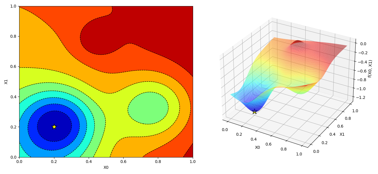
1. Multimodality: The inverted Franke function has two basins close to each other, making it a simple test for local minima avoidance.
2. Global minimum: The global minima is $f(x^*=<0.2,0.2>)=-1.2185807.$
3. Search space: The function is generally evaluated within the bounded region $[0, 1]$ for both $x$ and $y$.
4. Smoothness: The Franke function is very smooth so it is a good initial test for gradient-based algorithms due to its simplicity.

Discussion

It is commonly used as a test for interpolation and surface fitting functions, but we include it for its simplicity. It can serve as a follow-up to Sphere's (click here) unimodal landscape. Failures on this function indicate that the algorithm's exploration capabilities are weak.

Sources

The Franke function was introduced by Richard Franke in his 1979 paper titled A Critical Comparison of Some Methods for Interpolation of Scattered Data (click here).