Notebooks

Notebooks

The Notebook tab is a Jupyter-style editor built into ChipWhisperer Studio. You write Python cell by cell, run each cell and see its output, errors and plots underneath. Unlike a separate Jupyter server, notebook code shares Studio's hardware connection: cw.scope() and cw.target() give you the devices connected on the Connect tab, and every trace you capture appears live in the waveform view and the Capture tab. NewAE's own tutorial notebooks run unmodified.

The Notebook tab: files, tutorials and variables on the left, the notebook itself in the main area.

Creating and opening notebooks

The Notebooks card on the left lists every notebook in Studio's notebooks folder, grouped by sub-folder (click a folder name to expand it). Click a notebook to open it in a new tab (or switch to its tab if it is already open). The notebooks you had open, and how they were arranged, reopen when you return.

Action	How
New notebook	New, then type a name. It starts with a short example (connect, capture 50 traces).
Import an .ipynb	Import and pick the file. It is copied into the imported/ folder.
Save	Automatic 2.5 seconds after every change, when a cell finishes, and when you close the page. Save or Ctrl+S (Cmd+S on macOS) saves immediately. The toolbar shows unsaved or saved.
Export	The download button at the right of the toolbar saves the .ipynb through your browser, ready to open in Jupyter.
Rename	Double-click the notebook's tab and type a new name (a name with / moves it into a sub-folder). Its variables are kept.
Delete	Hover a notebook in the list and press its bin icon. An open notebook's tab closes.

Notebooks are standard Jupyter .ipynb files (nbformat 4), so they move freely between Studio and Jupyter.

Tabs and side by side

Every open notebook gets a tab above the notebook area. A tab shows the notebook's name and a dot: grey while it has unsaved changes, blue while its cells wait in the queue, amber (blinking) while one of its cells runs. Click a tab to show it, drag it along the tab bar to reorder, double-click it to rename, and press its x (or middle-click it) to close it.

To see two notebooks at once, split the notebook area into a left and a right pane, each with its own tabs:

Action	How
Split	Press the split button at the right end of the tab bar (it moves the current notebook into a new pane on the right), or drag a tab onto the right half of the notebook area. You can also drag a notebook from the Notebooks list onto a pane.
Move a notebook to the other pane	Drag its tab onto the other pane (onto its tab bar to choose the position), or press the arrows button at the right end of the tab bar.
Resize	Drag the bar between the panes; double-click it to make both panes equal.
Unsplit	Close or move away the last tab of a pane; the other pane takes the whole area.

Two notebooks side by side: each pane has its own tabs, and each notebook its own kernel and variables.

The pane you last clicked or typed in is the focused pane; its current tab is marked with a green line. Notebooks you open from the list open there, the Variables card shows that notebook's variables, and Ctrl+S saves it. Keyboard shortcuts in a cell always act on the notebook the cell belongs to. In a narrow window (below about 900 pixels) the panes are stacked, one above the other, and narrow panes show their toolbar buttons as icons only (hover a button for its name).

Cells

There are two kinds of cell:

• Code cells hold Python. The number in brackets on the left is the execution count: [3] means it was the third cell run since the kernel started, [*] means it is running, [ ] means it is queued.
• Text cells hold Markdown (headings, lists, tables, links, images, code blocks). They are shown formatted; double-click one to edit it, and press Shift+Enter or Esc to show it formatted again.

Hover a cell (or select it) to see its tools on the right: run, move up, move down, switch between code and text (M / Py), and delete. Add cells with + Code and + Text in the toolbar (inserted below the selected cell) or the buttons at the end of the notebook.

Keys

Key	In a cell
Shift+Enter	Run the cell and move to the next one (adds a new code cell at the end).
Ctrl+Enter (Cmd+Enter)	Run the cell and stay on it.
Alt+Enter	Run the cell and insert a new code cell below.
Enter	New line, keeping the indentation; one more level after a line ending in :.
Tab	Insert four spaces.
Esc	Leave the editor (and format a text cell).
Ctrl+S (Cmd+S)	Save the notebook in the focused pane.

Studio's single-key shortcuts (S, R, Esc, Space, + and -) do nothing while a notebook has the focus (you are in a cell or clicked in the notebook), so a key pressed after leaving a cell never starts a capture by accident; use the Single and Run buttons in the top bar.

Running code

Toolbar button	What it does
Run	Runs the selected cell and moves on (like Shift+Enter).
Run all	Runs every code cell from the top, in order. If a cell fails, the remaining queued cells are cancelled, as in Jupyter (they keep their previous execution count).
Stop	Interrupts this notebook's running cell (it ends with KeyboardInterrupt) and clears its queued cells. Other notebooks keep running.
Restart	After confirmation, clears this notebook's variables. Other notebooks are not affected and Studio stays connected to the hardware.
Power button	Shut down kernel: after confirmation, frees this notebook's variables and memory. A new, empty kernel starts when you run a cell.
Clear outputs	Removes all outputs and execution counts from the notebook.
View N traces	Appears when cells captured traces; jumps to the Capture tab.

The badge on the right shows Kernel idle, Running (with the number of this notebook's queued cells), Queued when its cells wait for another notebook's cell, or No kernel before the notebook has run anything.

One kernel per notebook

As in Jupyter, every notebook has its own Python session (its kernel): a variable defined in one notebook is not visible in another, each notebook counts its own executions ([1], [2], ...), and Stop, Restart and the Variables card apply to one notebook only. A notebook's kernel starts when it first runs a cell and moves with the notebook when you rename it.

All kernels share Studio's hardware connection, trace store and studio helper, so two notebooks talk to the same scope and target. Their cells go through one queue and run one at a time, in the order you ran them, on Studio's hardware thread: while a cell of one notebook runs, cells of the others wait (their badge says Queued). Each cell runs with its notebook's folder as the working directory, so relative paths work as they do in Jupyter.

When you close a notebook in every Studio window, its kernel is shut down about 20 seconds later (long enough to survive reloading the page) and its memory is freed. Kernels started from the HTTP API or MCP for notebooks that are not open stay until they are shut down.

Outputs

Output	How it is shown
print() and other text	Streamed while the cell runs. Progress bars (tqdm) update in place; colour codes are removed. Text written to stderr has an amber background. Very long outputs show their last 100,000 characters (download the notebook for all of it).
The value of the last line	Shown like in Jupyter, unless it is None (or a matplotlib object).
Errors	The traceback in red.
matplotlib figures	Every open figure is shown as an image when the cell finishes, and plt.show() shows the current figures immediately, so output before and after it stays in order.
display(obj)	Rich output: HTML, Markdown, PNG, JPEG or SVG when the object provides it, text otherwise.
HTML	Shown in a sandbox where scripts cannot run, so saved outputs from imported notebooks cannot interfere with Studio.

Variables

The Variables card lists the variables defined in the focused notebook (its name is shown next to the title): name, type (with the shape of arrays) and a short value. It refreshes after every cell of that notebook and when you focus another notebook; press Refresh to update it by hand.

Changes from other windows and agents

A notebook can be open in several Studio windows, and the HTTP API and MCP can run or rewrite it while it is open. Every save is announced to all windows:

• A tab without unsaved edits reloads the new version by itself (keeping its scroll position), for example after notebook_run saved its outputs.
• A tab with unsaved edits shows a notice instead of being overwritten: This notebook was changed outside this tab ... Nothing is saved until you choose. Choose Reload from disk or Keep my version.
• If the notebook was deleted or renamed elsewhere, a tab with edits offers Save it again or Close; a tab without edits closes. A rename in one window renames the tab in the others.

Saves never overwrite a newer version silently, and autosave never re-creates a deleted notebook.

Using the hardware from a notebook

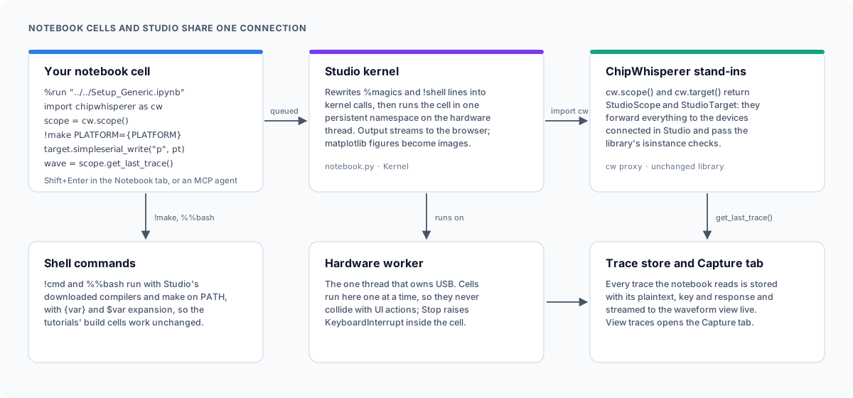
Notebook cells run on Studio's hardware thread and use the same scope and target as the rest of the app; every notebook has its own namespace.

Cells run on the same thread that talks to the ChipWhisperer, in turn with the rest of Studio, so the USB device is never used twice at once. Inside a notebook, import chipwhisperer as cw gives you the normal library with a few functions adapted to Studio:

Call	In a Studio notebook
cw.scope()	Returns Studio's connected scope. If none is connected, Studio connects one first: the simulator when Studio was started with --simulate, otherwise auto-detect. name= (for example "Husky") and sn= are honoured when connecting.
cw.target(scope, target_type)	Returns Studio's connected target, connecting it if needed (SimpleSerial v2 by default, the type you pass otherwise, the simulated target when the scope is the simulator).
cw.capture_trace(scope, target, text, key)	Captures as usual and also stores the trace in Studio.
cw.program_target(scope, prog, path)	Programs the target. With the simulator, an ELF (or a .hex Studio built, which has its .elf next to it) runs in the emulator from then on (Simulator: ... runs in the emulator); any other file is only checked to exist (Simulator: pretending to program ...).
cw.plot(trace)	Returns a plot that is drawn inline with matplotlib and also shows the trace in Studio's waveform view. Like ChipWhisperer's holoviews version, plots combine with * or + (cw.plot(a) * cw.plot(b)), cw.plot() with no data starts an empty plot to add to, and .opts(title=..., width=..., height=...) is accepted.
everything else	Unchanged: cw.ktp, cw.targets, cw.programmers, cw.analyzer and so on.

The scope and target you get are thin stand-ins (their type is StudioScope and StudioTarget) that forward everything to the device Studio is connected to at that moment. isinstance(scope, ...) checks behave as for the real object, settings work as usual (scope.gain.db = 25, scope.adc.samples = 5000), and they keep working if you reconnect in the Connect tab.

How traces reach the Capture tab

• Every trace returned by cw.capture_trace() is added to Studio's trace store with its plaintext, ciphertext and key.
• Manual capture loops, as used in many tutorials, work too: when the notebook calls scope.get_last_trace(), the trace is stored with the plaintext and key most recently sent with target.simpleserial_write('p', ...), target.simpleserial_write('k', ...) or target.set_key(). The ciphertext is filled in when the notebook reads the response with target.simpleserial_read().

The waveform view updates live while the cell runs. Afterwards, the View N traces button takes you to the Capture tab, and you can export the traces or run a CPA attack on them. Call studio.store_traces(False) to stop storing notebook captures.

Note: While a cell runs, it has the hardware thread to itself. Actions in other tabs that use the hardware (connecting, changing settings, Single, Run) wait until the cell finishes. Use Stop to interrupt a long cell.

The studio helper

Every notebook has a studio object:

Member	What it does
studio.traces	The stored traces. len(studio.traces), studio.traces[i] gives (wave, textin, textout, key), and .waves, .textins, .textouts, .keys give 2-D NumPy arrays of all traces.
studio.add_trace(wave, textin=None, textout=None, key=None)	Stores any 1-D array as a trace, so it appears in the waveform view and Capture tab. Returns its index.
studio.clear_traces()	Deletes all stored traces.
studio.show(wave)	Shows an array in the waveform view without storing it.
studio.store_traces(enabled=True)	Turns automatic storing of notebook captures on or off.
studio.build_firmware(project="simpleserial-aes", platform="CWLITEARM", compiler="gcc", **options)	Builds firmware exactly like the Firmware tab (options such as crypto_target, ss_ver, cflags, make_args, clean) and returns the .hex path. Raises an error with the end of the build log if the build fails. ss_ver defaults to SS_VER_2_1 like the Firmware tab; other options you leave out use the makefile's defaults.
studio.program(hex_path=None, programmer=None)	Programs the target, by default with the last build and its platform's programmer.
studio.session	Studio's internal session object, for advanced use.

hexfile = studio.build_firmware("simpleserial-aes", "CWLITEARM", crypto_target="TINYAES128C", ss_ver="SS_VER_2_1")
studio.program(hexfile)
waves = studio.traces.waves
print(waves.shape, waves.mean())

IPython features

Studio supports the IPython syntax that ChipWhisperer's notebooks use. Line magics and ! commands work wherever a statement starts, including inside loops and if blocks (but not inside brackets or strings, so % and ! keep their Python meaning there). Cell magics must be the first line of the cell.

Syntax	What it does
%run file.ipynb	Runs every code cell of another notebook in the current namespace (paths relative to the working directory, quotes allowed).
%run script.py	Runs a Python file in the current namespace.
!command	Runs a shell command and shows its output. Studio's installed compilers and make are on PATH, and the compatibility flags are in CFLAGS.
{expr} and $name in ! commands	Replaced by the value of a Python expression or variable, for example !make PLATFORM={PLATFORM} -j{n}. Write {{, }} or $$ for literal characters.
files = !ls	Runs the command and stores its output lines in a list.
%%bash (or %%sh)	Runs the whole cell with bash (or sh). %%bash -s "$PLATFORM" "{x}" passes the values as $1, $2, ...
%%script name	Runs the cell with the given interpreter.
%cd folder, %pwd	Change (and print) and show the working directory. A %cd lasts until the kernel restarts.
%env, %env NAME, %env NAME=value	Show all environment variables, one, or set one.
%time statement, %%time	Time one statement or the whole cell.
%timeit statement	Run a statement 7 times and print the average time.
%who, %whos	List variables.
%pip ..., %conda ...	Run pip in Studio's Python (%conda runs pip too). Not available in the standalone downloads.
%sx command, %system command	Run a command and return its output lines.
%%capture [name]	Run the cell without showing its output; store the output text in name.
%%writefile [-a] file	Write (or append) the cell's text to a file.
%%html, %%markdown	Show the cell as HTML or formatted Markdown.
name? or name??	Show help for an object.
%config InlineBackend.figure_format = 'svg'	Shows figures as SVG instead of PNG (retina, jpeg and pdf give PNG). Other %config settings are ignored.
%matplotlib, %load_ext, %reload_ext, %autoreload, %aimport, %precision, %xmode, and similar	Accepted and ignored, so notebooks written for Jupyter run unchanged.

Other magics raise UsageError: ... is not supported in Studio notebooks. ! commands run in your system's shell (cmd.exe on Windows). %%bash uses bash, or sh if bash is missing; on Windows install GNU make + sh on the Toolchains card to get sh.

Also available: display(), from IPython.display import display, HTML, Markdown, Image, SVG, clear_output, from tqdm.notebook import trange, tqdm (progress bars) and get_ipython() for run_line_magic, run_cell_magic, system and getoutput.

ChipWhisperer tutorials

The ChipWhisperer tutorials card downloads NewAE's tutorial notebooks, the chipwhisperer-jupyter repository with the SCA101, SCA201, Fault101 and other courses plus demos. Press Download tutorials.

• Studio downloads the version of chipwhisperer-jupyter that matches your firmware sources: the commit the ChipWhisperer repository pins for its jupyter submodule. If you have no firmware sources yet, it uses your channel's current commit.
• The notebooks go into <data dir>/notebooks/chipwhisperer-jupyter/ and appear in the Notebooks list.
• Studio links <data dir>/notebooks/firmware/mcu to the firmware sources (a symbolic link, or a directory junction on Windows), because the tutorials build firmware from ../../../firmware/mcu. If the firmware sources are not downloaded yet, the card reminds you to download them first.
• Downloading again updates the tutorials and keeps your work: files you edited or added are left alone. If a file you edited also changed upstream, Studio lists them and asks: Update, back up mine installs the new version and keeps yours next to it as <name>.local-YYYYMMDD-HHMMSS.ipynb, Keep mine leaves your copies as they are and updates everything else, and Cancel changes nothing.

NewAE's Lab 3_3 running in Studio: setup, firmware build, programming and capture.

Walkthrough: Lab 3_3, DPA on firmware AES

NewAE's labs come in parts: a (MAIN) notebook with the exercise (it contains raise NotImplementedError(...) placeholders for you to replace), and (HARDWARE) and (SIMULATED) notebooks that do the capture. The MAIN notebook defines a few settings and then runs the HARDWARE notebook with %run. The quickest way to see the capture work in Studio is to run the HARDWARE notebook directly with those settings:

1. On the Firmware tab, download the firmware sources and install the GNU Arm GCC toolchain.
2. Connect the scope and target on the Connect tab (or start Studio with --simulate to use the simulator).
3. On the Notebook tab, press Download tutorials.
4. Open chipwhisperer-jupyter/courses/sca101 and then Lab 3_3 - DPA on Firmware Implementation of AES (HARDWARE).
5. Select the first cell and add a code cell above it (or edit the first, empty code cell) with the settings the MAIN notebook would define, changing PLATFORM to match your target:

   SCOPETYPE = 'OPENADC'
   PLATFORM = 'CWLITEARM'
   CRYPTO_TARGET = 'TINYAES128C'
   SS_VER = 'SS_VER_2_1'

6. Press Run all.

What happens: %run "../../Setup_Scripts/Setup_Generic.ipynb" connects through Studio, the %%bash cell builds simpleserial-aes with Studio's compiler, cw.program_target flashes it (with the simulator, the firmware then runs in the emulator), and the capture loop records 2500 traces with a progress bar. The traces appear in the Capture tab with their plaintexts and keys; you can run Studio's own CPA attack on them. To do the full exercise, work through the MAIN notebook, which uses trace_array and textin_array from the capture.

Limitations

• holoviews and bokeh are not included. Tutorial cells that only use cw.plot() work through Studio's stand-in, but cells that import holoviews or bokeh directly fail with an import error; use matplotlib instead.
• Editing is a plain text editor: no syntax colouring and no autocomplete.
• One cell at a time: a running cell holds the hardware thread; other hardware actions in Studio, and cells of other notebooks, wait until it finishes.
• input() is not supported; set values in code instead.
• Stop raises KeyboardInterrupt in the running code. If the code is waiting inside a USB call, the interrupt takes effect when that call returns.
• Two panes at most side by side; use tabs for more notebooks.
• scope.dis() in a notebook disconnects Studio's scope too (it is the same device); reconnect on the Connect tab.

Where notebooks are stored

Path	Contents
<data dir>/notebooks/	Your notebooks (sub-folders allowed).
<data dir>/notebooks/imported/	Notebooks added with Import.
<data dir>/notebooks/chipwhisperer-jupyter/	NewAE's tutorials.
<data dir>/notebooks/firmware/mcu	Link to the firmware sources, for the tutorials.

The data folder is ~/ChipWhispererStudio unless you start Studio with --data-dir.

From the API and MCP

Action	HTTP API	MCP tool
List notebooks and tutorial status	GET /api/notebooks	notebook_list
Read / write a notebook	GET / PUT /api/notebooks/file	notebook_read / notebook_write
Run code and wait for the output	POST /api/kernel/run with {"code": "...", "kernel": "lab/a.ipynb"}	notebook_run_code with notebook_path
Run a whole notebook (in its own kernel) and save its outputs	POST /api/notebooks/run with {"path": "..."}	notebook_run
Queue cells (as the UI does)	POST /api/kernel/execute with kernel
Variables, interrupt, restart	GET /api/kernel/variables, POST /api/kernel/interrupt, POST /api/kernel/restart, each with an optional kernel	kernel_variables, kernel_interrupt, kernel_restart, each with an optional notebook_path
List and shut down kernels	GET /api/kernels, POST /api/kernels/shutdown	kernel_list, kernel_shutdown
Rename a notebook (its kernel follows)	POST /api/notebooks/rename
Download or update the tutorials	POST /api/notebooks/tutorials/fetch (on_modified: backup or keep after a confirm)	tutorials_fetch

A notebook's kernel id is its path relative to the notebooks folder. Without a kernel id, the API and MCP tools use a shared default kernel that no notebook tab uses, as before. See HTTP API and MCP Server.