Understanding Xdyn
Xdyn is the physics engine LOTUSim uses by default to simulate rigid-body motion in water. It's a lightweight opensource simulator developed by Sirehna (full documentation, French only), which LOTUSim adapts with a few integration specific changes.
This page covers how xdyn works conceptually, the physics behind it, and how it extend xdyn's own codebase. For practical .yml configuration, see Xdyn Setup. For the catalog of force/propeller types, see Forces & Propulsion (Xdyn).
- What Xdyn does
- The physics: Fossen's equation
- The default forces, explained
- Reference frames & conventions
- Units
- Command line usage
- Xdyn as a server
- Outputs
- Defining bodies: technical reference
- Wave & wind models: technical reference
- Wave presets in LOTUSim
- LOTUSim-specific changes
- Xdyn's codebase architecture
- Extending Xdyn's codebase
- Compiling & CI
- Development prospects
Xdyn solves the equations of motion for one or more rigid bodies in a fluid environment, over time. The forces acting on each body come from models either built-in (gravity, buoyancy, damping, propellers...) or user-supplied.
The physical problem (bodies, forces, environment) is described in a YAML input file; simulation parameters (time step, solver, duration) are set on the command line. This separation lets you re-run the same scenario with different solvers or durations without touching the YAML.
Xdyn implemented Fossen's equation of motion for marine vessels:
Where:
-
$\nu = (u,v,w,p,q,r)^T$ : the body's linear and angular velocity -
$M_A$ : added-mass matrix -
$C_A$ : Coriolis and centripetal matrix -
$D$ : damping matrix -
$g_0$ ,$g_b$ : restoring forces from gravity and buoyancy -
$\tau$ : control forces and torques (propellers, rudders...)
Each term on the right-hand side corresponds to a force model you add in its .yml file (see Xdyn Setup), the sum of everything you configure is what xdyn solves for at each time step.
Further reading: MSS (Marine Systems Simulator), Mathematical Ship Modeling for Control Applications.
Xdyn Setup and Forces & Propulsion (Xdyn) cover how to add these to your model. This section covers what they actually compute; useful when deciding which forces your model needs, or debugging why a force behaves the way it does.
Gravity - only uses g and the body's inertia matrix M
- model: gravity
Hydrostatic (buoyancy) - computed as:
where V is the immerged volume, calculated from the model's STL mesh, applied at the centre of buoyancy. This is what non-linear hydrostatic (fast) and non-linear hydrostatic (exact) compute → the "fast" variant trades some precision for speed.
- model: non-linear hydrostatic (fast)
Damping - a dissipative force from fluid shear on the hull, usually quadratic in vessel velocity (occasionally linear). Be mindful for double-counting: if you're also using radiation damping (below), don't let it overlap with your damping matrix. They represent different physical effects but can double-count energy dissipation if misconfigured.
- model: linear damping
  linear matrix at the center of gravity projected in the body frame:
    row 1: [ 0, 0,     0,      0,      0, 0]
    row 2: [ 0, 0,     0,      0,      0, 0]
    row 3: [ 0, 0, 1.9e5,      0,      0, 0]
    row 4: [ 0, 0,     0, 1.74e4,      0, 0]
    row 5: [ 0, 0,     0,      0, 4.67e6, 0]
    row 6: [ 0, 0,     0,      0,      0, 0]
- model: quadratic damping
  damping matrix at the center of gravity projected in the body frame:
    row 1: [ 0, 0,     0,      0,      0, 0]
    row 2: [ 0, 0,     0,      0,      0, 0]
    row 3: [ 0, 0, 1.9e5,      0,      0, 0]
    row 4: [ 0, 0,     0, 1.74e4,      0, 0]
    row 5: [ 0, 0,     0,      0, 4.67e6, 0]
    row 6: [ 0, 0,     0,      0,      0, 0]
Froud-Krylov (surface vessels only) - the force of the wave on the hull, assuming the ship doesn't perturb the wave itself.
-
non-linear Froude-Krylovintegrates the wave's pressure field over the hull mesh directly (using the STL file).
- model: non-linear Froude-Krylov
-
linear Froude-Krylovinstead uses precomputed Froude-Krylov forces and moments per frequency and direction from an HDB (hydrodynamic database) file, expressed at the centre of buoyancy.
- model: linear Froude-Krylov
  hdb: test_ship.hdb
  calculation point in body frame:
      x: {value: 0.696, unit: m}
      y: {value: 0, unit: m}
      z: {value: 1.418, unit: m}
  mirror for 180 to 360: true
  use encounter period: true
Diffraction (surface vessels only) - represents how the ship itself modifies the pressure field, e.g. the diffraction of the swell off the hull. Requires an RAO (Response Amplitude Operator), calculated per frequency and direction, from the same HDB file used for linear Froude-Krylov.
- model: diffraction
  hdb: test_ship.hdb
  calculation point in body frame:
      x: {value: 0.696, unit: m}
      y: {value: 0, unit: m}
      z: {value: 1.418, unit: m}
  mirror for 180 to 360: true
  use encounter period: true
Radiation damping (surface vessels only) - the energy dissipated by the vessel's own wave creation as it moves. Linear with respect to speed; requires the radiation damping terms from an HDB or PRECAL file. This is a more physically complete alternative/complement to linear damping/quadratic damping for vessels with wave data available.
- model: radiation damping
  hdb: test_ship.hdb
  type of quadrature for cos transform: simpson
  type of quadrature for convolution: clenshaw-curtis
  nb of points for retardation function discretization: 50
  omega min: {value: 0, unit: rad/s}
  omega max: {value: 30, unit: rad/s}
  tau min: {value: 0.2094395, unit: s}
  tau max: {value: 10, unit: s}
  output Br and K: true
  remove constant speed: true
  forward speed correction: true
Surface-force models (Froude-Krylov, diffraction, radiation damping) only apply to vessels operating at or near the surface - don't add them to a fully submerged model like an AUV.
NED (North-East-Down) is the fixed world reference frame, with a reference point
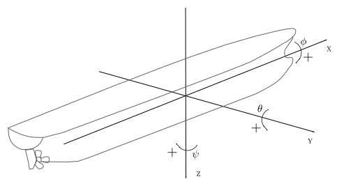
Body frame is attached to the vessel, generally centered at its center of gravity, with X forward, Y starboard, Z down. The equations of motion are solved in this frame.
Local NED is a frame centered on the vessel but with fixed (non-rotating) axes - used for exporting wave data near a moving vessel, where pure NED or pure body-frame coordinates are both awkward.
Generic frame definition - any reference frame in xdyn is defined relative to a known frame (NED or body) using this pattern, which shows up throughout the YAML file (e.g. position of body frame relative to mesh, initial position of body frame relative to NED):
frame: NED
x: {value: 0, unit: m}
y: {value: 0, unit: m}
z: {value: 0, unit: m}
phi: {value: 0, unit: rad}
theta: {value: 0, unit: rad}
psi: {value: 0, unit: rad}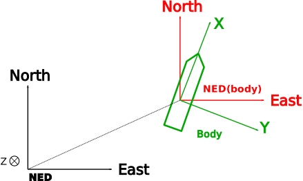
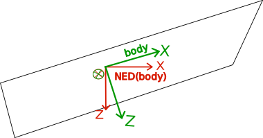
This reference frame is named “NED(body)”. Thus, if the ship is called “nav1”, the local NED reference frame will be “NED(nav1)”.
Orientation is described by a (phi, theta, psi) angle triplet. The convention is set once, in the rotations convention section:
rotations convention: [psi, theta', phi'']Apostrophes indicate that each subsequent rotation is composed relative to the new axis system from the previous rotation (an internal/intrinsic composition). So [psi, theta', phi''] means: rotate psi around Z, then theta around the new Y (Y'), then phi around the resulting X (X'').
The list always has three elements; the second is always different from the first, and the third is either different from both or equal to the first. A few named conventions:
| Convention | YAML |
|---|---|
| Aeronautical angles (yaw/pitch/roll - commonly, if imprecisely, called "Euler angles") | [psi, theta', phi''] |
| ParaView | [psi, phi', theta''] |
Don't change this from [psi, theta', phi''] → it's the only convention LOTUSim currently supports.
Quaternions are used internally to avoid gimbal lock and angle discontinuities, but Euler angles (phi, theta, psi) are what you'll typically read/write in configuration and output.
Each body's motion is fully described by 13 states:
| Symbol | Meaning | Unit |
|---|---|---|
| Position relative to the NED origin, projected into the body frame | m | |
| Attitude (see rotation convention above) | rad | |
| Quaternion form of attitude - used internally for integration | – | |
| Translation velocity relative to NED, projected into the body frame | m/s | |
| Rotation velocity of the body frame relative to NED, projected into the body frame | rad/s | |
| Forces applied to the ship, projected into the body frame | N | |
| Moments applied to the ship, projected into the body frame | N·m |
Xdyn is multi-body: several mechanically independent bodies can be simulated simultaneously, including their hydrodynamic interactions, provided an interaction model (which can come from a multibody HDB file) is implemented. Currently, no interaction forces or kinematic links are implemented.
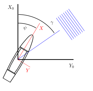
Xdyn uses the convention Z downward for wave amplitude. The azimuth/direction
The ship's position relative to the swell, as a function of
| Swell direction relative to ship | |
|---|---|
| 0° | Astern (following seas) |
| 0°–90° | Port quarter |
| 90° | Port beam |
| 90°–180° | Starboard aft |
| 180° | Bow (head seas) |
| 180°–270° | Starboard forward |
| 270° | Starboard beam |
| 270°–360° | Port forward |
Lines like this appear throughout the YAML file:
key: {value: 65456, unit: km}Units are not checked for physical consistency. The parser simply converts every value to SI units before simulation, using a multiplicative factor looked up from the UNIX units utility's unit list. It does not verify that the unit makes sense for the field. For example:
mass: {value: 10, unit: lb}is interpreted by xdyn as mass = 4.5359237 (kg). But this:
key: {value: 65456, unit: km}would produce exactly the same numeric result if you wrote unit: kW instead, even though kilometers and kilowatts are physically unrelated. Xdyn trusts that you've entered the value with a unit that's actually correct for that field; it only handles the conversion, not the validation.
If xdyn doesn't recognize a unit at all, it errors clearly (e.g. unknown unit: hhm), but a wrong-but-recognized unit will silently produce a wrong (converted) number. Double-check your units, especially copy-pasting between fields.
Run a simulation with a 4th-order Runge-Kutta solver:
./xdyn tutorial_01_falling_ball.yml --dt 0.1 --tend 1Use the Euler solver starting from a specific time:
./xdyn tutorial_01_falling_ball.yml -s euler --dt 0.1 --tstart 1 --tend 1.2Send output to standard output for piping into another process:
./xdyn scenario.yml --dt 0.1 --tend 1 -o csv | python plot.pyTo launch with grpc, where --port is where the websocket server listens:
./xdyn-for-cs --grpc --port 9002 tutorial_01_falling_ball.yml --dt 0.1Beyond running standalone, xdyn can run as a server so other simulation environments (Matlab, Simulink, custom tools) can drive it. This is what LOTUSim itself uses (xdyn-for-cs, see Getting Started and Xdyn Setup).
Two modes:
| Mode | Executable | What xdyn returns |
|---|---|---|
| Model exchange | xdyn-for-me |
State derivatives only - the client integrates |
| Co-simulation | xdyn-for-cs |
Fully integrated next state(s) - xdyn does the integration |
Both support JSON+WebSocket (default) or gRPC (--grpc, faster binary protocol) transport.
./xdyn-for-cs --port 9002 scenario.yml --dt 0.1Co-simulation advances the state forward:
Input:
| Field | Type | Details |
|---|---|---|
Dt |
Strictly positive float | Simulation horizon in seconds. Runs from t0 (the last date in states) to t0+Dt, in steps of dt (set on the command line). t0 appears in both input and output. |
states |
List of State
|
History of states up to the current time. If your models don't need history, this can have a single element. |
commands |
Dictionary | Actuator state at t0 - most often the internal state (e.g. rudder angle, propeller RPM) of a controlled force model, whose dynamics you're simulating outside xdyn. |
requested_output |
List of strings | Values xdyn should compute and return, using the same syntax as the YAML output section. |
Example input:
{
  "Dt": 10,
  "states": [
    {"t": 0, "x": 0, "y": 8, "z": 12, "u": 1, "v": 0, "w": 0,
     "p": 0, "q": 1, "r": 0, "qr": 1, "qi": 0, "qj": 0, "qk": 0}
  ],
  "commands": {"beta": 0.1},
  "requested_output": [
    "Fz(gravity,body,NED)",
    "My(non-linear hydrostatic (exact),body,body)"
  ]
}
Output is a list of "augmented state" elements covering t0 to t0+Dt in steps of dt, with the same 13-state fields listed in Ship states above, plus any extra_observations you requested:
{
  "t": [10, 10.1],
  "x": [0, 0.0999968],
  "y": [8, 8],
  "z": [12, 12.0491],
  "extra_observations": {
    "Fz(gravity,body,NED)": [2.135e3, 2.135e3],
    "My(non-linear hydrostatic (exact),body,body)": [4.984e4, 5.247e4]
  }
}
The meaning of the Euler angles depends on the rotations convention set in your YAML. This output is provided for client applications only, it's not used internally by xdyn. Each float has a unique textual representation (different binary floats always produce different strings, and converting text→binary reproduces the original value exactly), but the reverse isn't guaranteed: text→binary→text may not reproduce the exact same string, only the same numeric value.
The gRPC interface itself is described by a .proto file, see the xdyn source repository for the current definition (cosimulation.proto).
Configure what xdyn exports either via the command line (-o csv, -o test.hdf5 - quick, but exports everything) or via the YAML output section (full control over exactly which values to export → see Xdyn Setup for config examples). This section is the full reference for what you can actually export.
<format> |
Description |
|---|---|
csv / <file>.csv
|
CSV — to stdout (-o csv) or a file (-o test.csv) |
tsv / <file>.tsv
|
TSV |
json / <file>.json
|
JSON |
<file>.hdf5 / .h5
|
HDF5 (used by Matlab); file output only |
ws <address> |
JSON over websocket — xdyn connects to <address> as a client (see xdyn-for-me/xdyn-for-cs) |
Command-line output isn't configurable in content, xdyn writes everything available. Use the YAML output section for control.
Assuming a body named TestShip:
| Var | Description | YAML name | Unit |
|---|---|---|---|
| x, y, z | Body frame position in NED (BODY/NED) |
x(TestShip) etc. |
m |
| u, v, w | Velocity in NED, projected in body frame |
u(TestShip) etc. |
m/s |
| p, q, r | Angular velocity around body axes |
p(TestShip) etc. |
rad/s |
| qr, qi, qj, qk | Orientation quaternion (BODY/NED) |
qr(TestShip) etc. |
– |
| phi, theta, psi | Roll, pitch, yaw |
phi(TestShip) etc. |
rad |
Add _filtered to any of these (e.g. q_filtered) for a filtered version - quaternions aren't filtered, but Euler angles are.
output:
  - format: csv
    filename: example.csv
data: [t, y_filtered(TestShip), theta(TestShip)]Force models that declare extra_observations expose additional exportable values:
| Model | Extra values |
|---|---|
| Hydrostatic |
Bx, By, Bz
|
| GM |
GM, GZ
|
| Hydrodynamic polar |
alpha, U
|
| gRPC models | Whatever the external model declares |
A Python gRPC model, for example, can return:
def force(self, states, commands, __):
    return {'Fx': 0, 'Fy': 0, 'Fz': 0, 'Mx': 0, 'My': 0, 'Mz': 0,
            'extra_observations': {'k': 2, 'harmonic_oscillator_time': states.t[0]}}
which then becomes accessible as 'harmonic_oscillator_time(TestShip)' in the output section.
Fx(model,body,reference), Fy(...), Fz(...), Mx(...), My(...), Mz(...) - in N / N·m.
-
model- the force'smodelname in YAML -
body- the body the force acts on -
reference-NED, the body's name, or the force model's own name if its parameterization includes aframekey (hydrodynamic polar,aerodynamic polar,maneuvering,wageningen B-series,propeller+rudder,Kt(J) & Kq(J),grpc) Special aggregate keys: -
Fx/Fy/Fz/Mx/My/Mz(sum of forces,body,reference)- total force/moment on the body -
Fx(blocked states,body,body)- force required to maintain a forced degree of freedom (only in the body's own frame) -
Fx(fictitious forces,body,reference)- Coriolis + centripetal forces, arising from the body frame's non-Galilean nature (see Fossen for the calculation) Example:
output:
  - format: hdf5
    filename: test.h5
    data: [Fx(gravity, ball, ball), Fy(gravity, ball, ball), Fz(gravity, ball, ball), Mx(sum of forces,ball,NED)]
Commands on force models that take them (propeller+rudder, maneuvering, etc.) are exportable as name(command):
output:
  - format: csv
    filename: propRudd.csv
data: [t, 'Prop. & rudder(rpm)', 'Prop. & rudder(beta)']| Key | Content |
|---|---|
mesh |
The STL mesh, in /inputs/meshes
|
yaml |
Concatenation of input YAML files, in /inputs/yaml/input
|
command line |
The launch command line |
matlab/python scripts |
Helper scripts for processing the HDF5 file, in /scripts/
|
waves |
Free surface elevation on the grid defined in the wave model's output section |
spectra |
Wave spectra, in /outputs/spectra/
|
output:
  - format: hdf5
    filename: test.h5
data: [mesh, 'command line']Xdyn Setup covers the quick version. This is the full field-by-field reference for the bodies section.
The mesh key is optional, but required for integrated hull forces (non-linear hydrostatic, Froude-Krylov). It points to an STL file (ASCII or binary), path relative to where the simulator is launched.
Orientation: xdyn ignores the normals stored in the STL file and recalculates them via the right-hand rule from each face's ordered points. Normals must point toward the fluid, xdyn warns if many faces seem oriented toward the mesh's barycenter, but this can be a false positive for complex (multi-shell) geometries, so it's worth double-checking manually.
Mesh frame → body frame: the body frame's origin is given relative to the mesh frame, x, y, z position the center of gravity in mesh coordinates, and phi, theta, psi give the rotation from mesh frame to body frame (per your rotations convention):
position of body frame relative to mesh:
    frame: mesh
    x: {value: 0, unit: m}
    y: {value: 0, unit: m}
    z: {value: -10, unit: m}
    phi: {value: 1, unit: rad}
    theta: {value: 3, unit: rad}
psi: {value: 2, unit: rad}Five subsections describe the body's inertia:
Hydrodynamic calculation point where viscous damping and forward-resistance forces are calculated, in a frame translated from the body frame. Its x is the center of the mesh's projection onto the (x,z) plane, y is zero, and z is the center of the mesh's projection onto the (x,y) plane, generally distinct from both the center of gravity and center of volume:
hydrodynamic forces calculation point in body frame:
    x: {value: 0.696, unit: m}
    y: {value: 0, unit: m}
    z: {value: 1.418, unit: m}
Don't confuse this with the separate reference frame used by HDB files for radiation damping matrices, force RAOs, and added masses.
Center of inertia (if different from the body frame's origin):
center of inertia:
    frame: TestShip
    x: {value: 0, unit: m}
    y: {value: 0, unit: m}
    z: {value: 0, unit: m}
frame can be NED, a body's name, or mesh(<body name>).
Mass:
mass: {value: 1000, unit: ton}
⚠️ tonis the British ton (907.185 kg), not the metric tonne.
Inertia matrix (not normalized; SI units, kg for the 3×3 translational block, kg·m² for the rotational block, kg·m for cross terms):
rigid body inertia matrix at the center of gravity and projected in the body frame:
    row 1: [253310,0,0,0,0,0]
    row 2: [0,253310,0,0,0,0]
    row 3: [0,0,253310,0,0,0]
    row 4: [0,0,0,1.522e6,0,0]
    row 5: [0,0,0,0,8.279e6,0]
    row 6: [0,0,0,0,0,7.676e6]
Optional key convention z down: true/false: defaults to true (xdyn's Z-down convention).
Added mass matrix : same format, but sits in dynamics rather than external forces, because it's applied on the left-hand side of
Can also be read directly from a database instead of declared inline:
added mass matrix at the center of gravity and projected in the body frame:
    from hdb: test_ship.hdb        # HDB: uses the matrix at the file's minimum period, no extrapolation
    # or:
    from raodb: ONRT_SIMMAN.raodb.ini   # PRECAL_R: infinite-frequency asymptotic value, no interpolation needed
If reading from a file, omit frame and row entirely, xdyn errors if you mix both to avoid ambiguity.
You can force u, v, w, p, q, r (velocities) per body, not position/attitude directly, since that would require also forcing the corresponding velocities and solving a minimisation problem for consistent quaternions.
blocked dof:
   from CSV:
     - state: u
       t: T
       value: PS
       interpolation: spline
       filename: test.csv
   from YAML:
     - state: p
       t: [4.2]
       value: [5]
interpolation: piecewise constant-
state: one ofu, v, w, p, q, r -
t/value: either inline arrays (YAML) or column names in a CSV file -
interpolation:piecewise constant,linear, orsplineOutside the range[tmin, tmax], the state is unforced. When forced, the derivative is forced too, before the solver runs; forces are recalculated using the forced state, then the state is forced again afterward so the forced values aren't integrated.
The force actually required to maintain the forcing : Fx/Fy/Fz/Mx/My/Mz(blocked states, TestShip, TestShip), expressed in the body frame.
Environment models (wave, wind, and current) are configured in environment models. Wave models feed non-linear hydrostatic forces (via free-surface elevation), Froude-Krylov forces (via dynamic pressure), diffraction forces (via frequency), and the rudder model (via orbital velocity). Wind models feed sail/wind-propulsion models.
environmental constants:
    g: {value: 9.81, unit: m/s^2}
    rho: {value: 1025, unit: kg/m^3}
    nu: {value: 1.18e-6, unit: m^2/s}
    air rho: {value: 1.225, unit: kg/m^3}   # optional - only needed for aerodynamic models
These four are currently the complete set of environmental constants xdyn uses.
environment models:
  - model: no waves
    constant sea elevation in NED frame: {value: 0, unit: m}
A flat, horizontal free surface - Froude-Krylov and radiation excitation forces are zero.
A wave is the sum of directional spectra (power spectrum × spatial dispersion). Assuming inviscid, incompressible, irrotational flow, velocity derives from a potential
where
Dispersion relation (relating
Wave elevation, generalised to multiple frequencies and directions (with
Dynamic pressure (used by Froude-Krylov):
Total pressure (hydrostatic + dynamic) can be shown to always be non-negative below the free surface, a useful sanity check on any custom wave model, though the full proof is a case-by-case algebraic argument not reproduced here.
Orbital velocity
At infinite depth (
Parameterisation:
- model: airy
  depth: {value: 100, unit: m}          # 0 = infinite-depth approximation
  seed of the random data generator: 0  # 'none' → all phases zero (useful for testing)
  stretching:
     delta: 0
     h: {unit: m, value: 100}
  directional spreading:
     type: dirac
     waves propagating to: {value: 90, unit: deg}
  spectral density:
     type: jonswap
     Hs: {value: 5, unit: m}
     Tp: {value: 15, unit: s}
     gamma: 1.2
Airy wave model as a list
You can describe the Airy wave model by a list of lines. To use this modeling, you must declare a section spectra from a list of rays in model: waves.
environment models:
  - model: waves
    spectra from a list of rays:
      - model: airy
        stretching:
           delta: 0.5
           h: {unit: m, value: 100}
        depth: {value: 1.7, unit: km}
        rays:
          # Two rays with T=8s and T=10s
          a: {values: [0.1, 0.5], unit: m}
          psi: {values: [180.0, 180.0], unit: deg}
          omega: {values: [0.628318, 0.785398], unit: rad/s}
          k: {values: [3.872832, 6.051301], unit: 1/m}
          phase: {values: [50, 90], unit: deg}
      - model: airy
        stretching:
           delta: 0.5
           h: {unit: m, value: 100}
        depth: {value: 1.7, unit: km}
        rays from file: rays.csv
The rays provided in a CSV file are described in international units with 5 columns, with:
- the amplitude
ain meters (which will generate oscillations between$-a$ and$+a$ ), - the direction of propagation
psiin radian, - the angular frequency
omegain rad/s, - the wave number
kin rad/m, - the phase
ain radian.
| Type | Formula | Notes |
|---|---|---|
dirac |
Single frequency |
Monochromatic, useful for transfer functions, not representative of real seas |
bretschneider |
|
General-purpose 2-parameter spectrum |
pierson-moskowitz |
Special case of Bretschneider ( |
Fully-developed seas only |
jonswap |
Limited fetch, North Sea storms — this is what LOTUSim's wave presets use |
spectral density: {type: jonswap, Hs: {value: 5, unit: m}, Tp: {value: 15, unit: s}, gamma: 1.2}| Type | Formula | YAML |
|---|---|---|
dirac |
Unidirectional | {type: dirac, waves propagating to: {value: 90, unit: deg}} |
cos2s |
{type: cos2s, s: 2, waves propagating to: {value: 90, unit: deg}} |
Airy's formulation isn't valid above h (height over which stretching applies) and delta (0–1):
| Model | Config |
|---|---|
| No stretching (not recommended with orbital-velocity-dependent models) |
h: {value: 0, unit: m}, delta: 1
|
| Linear extrapolation |
h = depth, delta: 1
|
| Wheeler stretching |
h = depth, delta: 0
|
There's no strong theoretical justification for any one stretching model over another, the choice is empirical, based on comparison with measured velocity profiles, and test campaigns haven't produced a definitive winner. Wheeler's model tends to underestimate orbital velocity at wave peaks.
discretization:
    nfreq: 128 # number of frequencies
    ndir: 8 # number of directions
    omega min: {value: 0.1, unit: rad/s} # min angular frequency (inclusive)
    omega max: {value: 6, unit: rad/s}
    energy fraction: 0.999
    equal energy bins: true
Only the energy fraction of total spectral energy is retained (sorted by contribution, descending), this keeps computation tractable, though it can miss low-energy components that matter for specific responses (wetness, slamming, appendage loads). equal energy bins: true discretizes frequencies so each bin's trapezoidal-integrated energy is equal, rather than spacing frequencies evenly.
Implement a wave model in any language (Python, Java, Go...) as a gRPC service, and use it from xdyn like a built-in model:
- model: grpc
  url: http://localhost:50001
  Hs: 5
  Tp: 15
  gamma: 1.2
Parameters are passed through to the server unparsed by xdyn.
Currently "static", vary with altitude, not time.
| Model | Formula | Config |
|---|---|---|
no wind (default) |
— | - model: no wind |
uniform wind |
Constant everywhere |
velocity, direction
|
power law wind profile |
alpha ≈ 0.11 at sea, 0.143 on land |
|
logarithmic wind profile |
|
roughness length |
Further reading: Wind profile power law; Log wind profile; Roughness length
Rather than requiring users to hand-tune wave spectra, LOTUSim's surface vessels currently use 10 preset sea states based on the World Meteorological Organization (WMO) scale, each a JONSWAP spectrum with
| Code | Wave height | Characteristics | Height (Hs) | Period (Tp) |
|---|---|---|---|---|
| 0 | 0 m | Calm (glassy) | 0 | 0 |
| 1 | 0 - 0.1 m | Smooth (wavelets) | 0.1 | 1 |
| 2 | 0.1 - 0.5 m | Calm (rippled) | 0.5 | 2 |
| 3 | 0.5 - 1.25 m | Slight | 1.5 | 3 |
| 4 | 1.25 - 2.5 m | Moderate | 4 | 4 |
| 5 | 2.5 - 4 m | Rough | 6 | 6 |
| 6 | 4 - 6 m | Very rough | 8 | 7 |
| 7 | 6 - 9 m | High | 11 | 8 |
| 8 | 9 - 14 m | Very high | 16 | 9 |
| 9 | Over 14 m | Phenomenal | 20 | 10 |
Further reading: Sea state (Wikipedia), Waves (Coastal Wiki), Wave period parametization, Wave period, Dominant wave period, Waves in the Ocean
On currents: ocean current velocity is physically a sum of several components (tidal, wind-generated, thermohaline, Stokes drift...) - modeling all of them is significantly more complex than the wave presets above. LOTUSim currently implements only the Ekman current model (see Forces & Propulsion (Xdyn) and Xdyn Setup); the fuller current model is a documented area for future work (see Development prospects).
LOTUSim renders the same wave elevation in both Xdyn (for physics) and Unity (for visuals, via the HDRP package), which requires the two to agree on how waves repeat in space.
In Xdyn: Unity's wave rendering works by tiling repeating squares of different sizes, each with a fixed number of points (its resolution). To make xdyn's wave output tile the same way, xdyn's waves are configured to be spatially periodic, with a period L equal to Unity's repetition size.
In Unity: all modifications relative to the stock HDRP package are marked with // CHANGES-FOR-UNITY comments in the source, so they're easy to find and diff against upstream Unity releases.
This section is for contributing to xdyn's own codebase (not LOTUSim's Gazebo-side plugins - see Extend with your components for those).
Xdyn's code is split into modules by two criteria: what the code does (each module is functionally coherent) and its dependencies (minimized between modules).
| Module | Description |
|---|---|
core |
Computational core describing simulator behaviour |
environment_models |
Wave models |
exceptions |
Error handling |
executables |
Main programs (xdyn-for-me, xdyn-for-cs, xdyn, gz) |
external_data_structures |
Data structures for values read from YAML |
external_file_formats |
Reading external files (HDB, STL) |
force_models |
Force models |
gz_curves |
Calculating GZ and GM |
hdb_interpolators |
Extraction of data from PRECAL_R and HDB (AQUA+) files |
interface_hdf5 |
Writing HDF5 files |
mesh |
Mesh calculations (ship/free-surface intersection, facet iteration) |
observers_and_api |
Output definitions during simulation (CSV, HDF5, websocket...) |
listeners_and_controllers |
Reading command files, controllers, and wave spectra |
test_data_generator |
Test data generation (used for tutorials) |
yaml_parser |
Generic YAML interpretation (bodies, outputs) |
wrapper_python |
Python interface to the xdyn API |
Each module has a CMakeLists.txt, an inc directory (headers), and optionally a unit_tests subdirectory.
From command line to results, the simulator: retrieves arguments → opens files (YAML + command files, read but not yet interpreted) → creates the system to be simulated (interprets file contents into internal data structures) → creates observers → runs the simulation.
The relevant files, all in the executables module:
-
simulator.cpp: containsmain -
utilities_for_InputData.cpp: reads the command line viaboost::program_options -
simulator_run.cpp: high-level orchestration of the steps above
Creating the system happens in two steps, both in simulator_api.cpp (observers_and_api module):
-
get_systemcalls the main YAML parser (SimulatorYamlParser), which builds aYamlSimulatorInputtree mirroring the whole input file. Notably, the parser does not interpret force/wave model YAML itself → that's stored as a string and parsed later by each model's own parser. This lets force models evolve independently without touching the shared parser. -
get_buildercreates the system viaSimulatorBuilder, which doesn't know about any specific force/wave model. It's configured with a list of parsers viacan_parse<T>():
SimulatorBuilder builder(yaml, t0, command_listener);
builder.can_parse<DefaultSurfaceElevation>()
       .can_parse<BretschneiderSpectrum>()
       .can_parse<JonswapSpectrum>();
For each model declared in YAML, every registered parser's try_to_parse is tried in turn until one succeeds (or none do, which is an error).
Environment construction (SimulatorBuilder::build_environment_and_frames): stores constants read directly from YAML, then builds the wave model and the Kinematics object used for reference-frame changes. Wave model construction (SimulatorBuilder::get_wave) retrieves a list of (name, YAML string) pairs, then tries each registered wave parser's try_to_parse on each - the same pattern used for all models (controlled and uncontrolled forces alike).
Force construction (SimulatorBuilder::get_forces): for each body, SimulatorBuilder::forces_from is called with the already-built environment model (each force model's constructor needs it). forces_from loops over the body's force models (name + YAML string) and calls SimulatorBuilder::add, which loops over all registered force parsers calling try_to_parse, returning boost::optional<ForcePtr>.
Bodies are constructed in SimulatorBuilder::build, simply invoking the Sim class constructor with everything built above (forces, environment, controls).
Sim::operator(), called by the solver's Stepper every step, does four things: updates each body's state/mesh, sums the forces on each body, calculates state derivatives, and normalizes quaternions.
Updating bodies: transforms NED↔BODY, records the new state, and (for surface bodies) recalculates the hull/free-surface intersection via MeshIntersector. The Body class is abstract (update_intersection_with_free_surface is pure virtual), with two subclasses: BodyWithSurfaceForces (does the mesh/free-surface work) and BodyWithoutSurfacesForces (doesn't). MeshIntersector is the most performance-critical, and consequently least readable, part of the codebase, especially MeshIntersector::split_partially_immersed_facet_and_classify. It's used by all surface force models (ExactHydrostaticForceModel, FastHydrostaticForceModel, GMForceModel) via SurfaceForceModel::operator().
Summing forces (Sim::sum_of_forces): centripetal/Coriolis forces, updates each force model with the new state, changes reference frames as needed, and sums.
State derivatives (Body::calculate_state_derivatives): since xdyn's integrator doesn't support constrained solving, forced states/derivatives are handled by the BlockedDOF class in two stages — forcing states (via Body::update_body_states), then forcing derivatives (via Body::calculate_state_derivatives).
Preparing observations (Sim::output): passes each observer through every force model and body to collect exportable values, and computes the difference between calculated and actually-applied forces (for forced states).
The simulation uses ssc::solver, a thin layer over boost::odeint, invoked in simulator_run.cpp:
ssc::solver::quicksolve<Stepper>(system, scheduler, observer);| Parameter | Description |
|---|---|
Stepper |
The solver, e.g. ssc::solver::EulerStepper (alias for boost::numeric::odeint::euler<std::vector<double>>) |
system |
Object exposing void operator()(x, dxdt, t) — here, the Sim class |
scheduler |
Derived from Scheduler
|
observer |
Derived from Observer
|
The solver's two jobs: call the observer at the end of each step, and advance system state step-by-step using the Stepper (which only needs state derivatives - Sim's responsibility to provide them).
Observers serialize simulation state (CSV, HDF5, TSV, JSON, websocket, plus std::map for internal unit tests) as the simulation runs. Design goals: support multiple parallel serializations, require only one code location to make a variable serializable, and require only one location to add a new serialization type.
The abstract Observer class (core module) has all pure virtual methods marked protected, so derived classes can't change call order. Two key design choices: initialization is separate from serialization, and virtual methods return functions to run later rather than performing work directly — which complicates changes to how the solver invokes serialization (touching both SSC and every observer), as happened when controllers and force serialization were added.
Workflow: the user defines serializations in the YAML output section → after system creation, run_simulation (simulator_run.cpp) creates observers via get_observers, which parses output into YamlOutput structures → command-line observers (-o) are appended → get_observers builds the final list via the ListOfObservers constructor.
ListOfObservers is itself an observer (in the ssc::solver::quicksolve sense) but doesn't derive from Observer — it just has observe_(before/after)_solver_step methods that call the corresponding method on each contained observer.
Timing matters: since observation only reads state (it doesn't call force models, to avoid costly recomputation), a memoization cache reuses force evaluations from just before observation to avoid double-evaluating them mid-step, relevant for multi-stage solvers like RK4, where an intermediate state (e.g.
Observer::observe_(before/after)_solver_step first makes the current time available via write, then requests all serialisable values via Sim::output, which calls each force model's and body's feed method (providing Fx, Fy, Fz, K, M, N, plus any extra_observations), nothing is actually written yet at this point. Actual serialization happens in two final calls: initialize_everything_if_necessary (once, before the first step) and serialize_everything (every step), which looks up each value's serialisation function (populated by earlier write calls) and invokes it.
- Create
.hpp/.cppinforce_models/incandforce_models/src; add a unit test inforce_models/unit_tests(strongly recommended) - Add both to their respective
CMakeLists.txt - Choose a base class:
ImmersedForceModel(submerged surface force, e.g. hydrostatic),EmergedForceModel(above-surface, e.g. wind), orForceModel(non-surface) - Document the model in
XDYN_ROOT/doc/user_en/modeles_efforts.md
Data available to your model: the current time, the environment (EnvironmentAndFrames - environmental variables plus wave/wind models), any required command values, and a BodyStates object containing the 13 body states, the mesh (if any), inertia matrices, quaternion-to-angle conversion helpers, a MeshIntersector for submerged/emerged facets, and a few specific points (dynamics resolution point, mesh frame center, hydrodynamic calculation point).
Every force model must implement:
-
static std::string model_name(): the name used in YAML - A constructor taking at least the body name and environment
Wrench get_force(const BodyStates&, const double, const EnvironmentAndFrames&, std::map<std::string,double>) const override
Optionally: double get_Tmax() if the model needs state history, and void extra_observations(Observer&) to export extra values beyond the force tensor.
Return format: get_force returns a Wrench — 3 force components, 3 moment components, the expression frame's name, and the application point (ssc::kinematics::Point). Your model can express the force in whatever frame/point is most convenient; the parent ForceModel class handles converting it to the body frame at the dynamics resolution point.
If your model uses its own custom expression frame, pass a YamlPosition (internal_frame) to the ForceModel constructor:
ForceModel(const std::string& name, const std::vector<std::string>& commands,
           const YamlPosition& internal_frame, const std::string& body_name_,
           const EnvironmentAndFrames& env);
If it uses a known frame (body, NED, mesh, local NED), skip YamlPosition:
ForceModel(const std::string& name, const std::vector<std::string>& commands,
           const std::string& body_name_, const EnvironmentAndFrames& env);
No parser needed (e.g. GravityForceModel) - the constructor must respect:
GravityForceModel(const std::string body_name, const EnvironmentAndFrames& env);Parser needed (e.g. GMForceModel) - implement a static parse, and have your constructor take its result as the first argument:
static Input parse(const std::string& yaml);
GMForceModel(const Input& input_data, const std::string body_name, const EnvironmentAndFrames& env);
The return type of parse must match the constructor's first parameter type.*
Controlled forces (need commands) pass a command list to the ForceModel constructor:
ForceModel(const std::string& name, const std::vector<std::string>& commands,
           const YamlPosition& internal_frame, const std::string& body_name_,
           const EnvironmentAndFrames& env);
ForceModel(const std::string& name, const std::vector<std::string>& commands,
           const std::string& body_name_, const EnvironmentAndFrames& env);
For example:
SimpleHeadingKeepingController::SimpleHeadingKeepingController(
    const Input& input_data, const std::string& body_name_, const EnvironmentAndFrames& env_) :
        ControllableForceModel(
            input.name,
            {“psi_co”}, // ‘psi_co’ is the only command needed by SimpleHeadingKeepingController
            YamlPosition(YamlCoordinates(),YamlAngle(), body_name_),
            body_name_,
            env_)
get_force then receives a dictionary of the requested command values (without the model name prefix). Pass {} if no commands are needed.
Register it - add a line to get_builder in simulator_api.cpp (observers_and_api module):
builder.can_parse<GravityForceModel>()
.can_parse<GMForceModel>();New output formats (e.g. CsvObserver) live in observers_and_api and derive from Observer, implementing:
void flush_after_initialization() override;
void flush_after_write() override;
void flush_value_during_write() override;
std::function<void()> get_serializer(const double val, const DataAddressing& address) override;
std::function<void()> get_initializer(const double val, const DataAddressing& address) override;
(Add using Observer::get_serializer; and using Observer::get_initializer; in the class declaration to avoid masking.)
For CsvObserver, get_initializer writes column headers, flush_after_initialization adds the line break after them, flush_value_during_write inserts a comma between values, flush_after_write adds the line break after the last value, and get_serializer writes each value:
std::function<void()> CsvObserver::get_initializer(const double, const DataAddressing& address) {
    return [this,address](){ std::string title = address.name; boost::replace_all(title, ",", " "); os << title; };
}
std::function<void()> CsvObserver::get_serializer(const double val, const DataAddressing&) {
    return [this,val](){ os << val; };
}
Register it in two places:
-
ListOfObserversconstructor (ListOfObservers.cpp) - mapsoutput.format(from YAML) to your observer class:if (output.format == "csv") observers.push_back(ObserverPtr(new CsvObserver(...))); -
build_YamlOutput_from_filename/get_format(parse_output.cpp,yaml_parsermodule) - maps a file extension to your format, so-o file.extpicks the right observer
Wave models (in environment_models module) are built from 3 types:
-
WaveSpectralDensity: power spectral density (e.g.JonswapSpectrum) -
WaveDirectionalSpreading: directional spreading (e.g.Cos2sDirectionalSpreading) -
WaveModel: combines a discretised spectrum (DiscreteDirectionalWaveSpectrum) + spreading into elevation, orbital velocity, RAO, and dynamic pressure (e.g.Airy)
Unlike force models, wave models aren't yet unified under one parsing pattern. Adding one touches five modules: environment_models (the model itself), external_data_structures (YAML data structure), listeners_and_controllers (parser interface), yaml_parser (actual parsing), and observers_and_api (registration in simulator_api.cpp).
Worked example - adding a power spectral density (JONSWAP):
- Create
JonswapSpectrum.hpp/.cppinenvironment_models; add aJonswapSpectrumTestunit test (recommended) - Derive from
WaveSpectralDensity, implementing:
double operator()(const double omega) const;
WaveSpectralDensity* clone() const { return new JonswapSpectrum(*this); }- Define a
YamlJonswapdata structure (inYamlWaveModelInput.hpp,external_data_structures) for the parsed YAML fields - Specialize
SpectrumBuilder<JonswapSpectrum>inlisteners_and_controllers(builders.hpp):
template <>
class SpectrumBuilder<JonswapSpectrum> : public SpectrumBuilderInterface {
public:
    SpectrumBuilder();
    boost::optional<TR1(shared_ptr)<WaveSpectralDensity>> try_to_parse(const std::string& model, const std::string& yaml) const;
};- Implement the actual YAML parsing (
parse_jonswap, inenvironment_parsers.cpp,yaml_parsermodule) and use it insidetry_to_parse:
boost::optional<TR1(shared_ptr)<WaveSpectralDensity>> SpectrumBuilder<JonswapSpectrum>::try_to_parse(
    const std::string& model, const std::string& yaml) const {
    boost::optional<TR1(shared_ptr)<WaveSpectralDensity>> ret;
    if (model == "jonswap") {
        const YamlJonswap data = parse_jonswap(yaml);
        ret.reset(TR1(shared_ptr)<WaveSpectralDensity>(new JonswapSpectrum(data.Hs, data.Tp, data.gamma)));
    }
    return ret;
}- Register it:
builder.can_parse<JonswapSpectrum>();inget_builder(simulator_api.cpp) Directional spreading (e.g.Cos2sDirectionalSpreading) follows the identical pattern, deriving fromWaveDirectionalSpreadingand specializingDirectionalSpreadingBuilder<T>instead ofSpectrumBuilder<T>.
A WaveModel must implement:
-
evaluate_rao- used for radiation damping -
elevation- used by hydrostatic models -
orbital_velocity- used byRudderForceModel -
dynamic_pressure- used for Froude-Krylov forces As with force models, finish by registering it:builder.can_parse<Airy>();
From a blank machine:
# From XDYN_ROOT/code
mkdir build && cd build
cmake ..              # or -G Ninja for faster builds; -G "MSYS Makefiles" on Windows/MinGW
make
./run_all_tests       # run unit tests
make doc               # build documentation
make package           # create an installation program
Helper scripts at the xdyn repo root:
| Script | Purpose |
|---|---|
gdb.sh |
Launch an executable under GDB (compile in debug mode first with ninja_debug.sh) |
ninja_debian.sh |
Compile in release mode (Linux) |
ninja_debug.sh |
Compile in debug mode (Linux) |
run_all_tests_debian.sh |
Run unit tests (Linux); supports Google Test flags |
run_all_tests_valgrind.sh |
Run tests under Valgrind to catch memory issues |
Git workflow: feature branches (a few dozen commits max, ~10 days max lifetime), linked to a GitLab issue. No direct commits to master. Every push triggers CI (compile, generate docs, run tests, code metrics, Valgrind, build installer). Once CI passes, a maintainer code-reviews the merge request; once comments are addressed and CI is green, it's merged to master. Developers rebase on master regularly during development.
Documented areas for future xdyn work:
Additional models: nonlinear regular wave model; wind (Harris spectrum); environmental conditions that vary over a scenario; unifying wave model parsing with the force-model pattern (currently touches 5 modules instead of 1); recognising output format from file extension automatically; second-order wave loads.
Multi-body: kinematic links (simulating linked/attached objects); collision detection; algebraic-differential system integration (to properly force states, not just derivatives).
Performance: faster mesh-intersection calculations (e.g. via GTS or CGAL, meshing the free surface and intersecting with the hull mesh rather than per-point wave height calculation); GPU-parallelized wave model evaluation; compiling maneuverability models natively instead of interpreting them.