Bleed Through Correction
Spectral bleed-through (cross-talk) is the signal that leaks from the donor and acceptor fluorophores into the FRET detection channel. It must be measured and removed before FRET efficiency can be calculated accurately. The Bleed-Through tab estimates the bleed-through coefficients from single-label control images and fits a correction model that the FRET tab then applies.
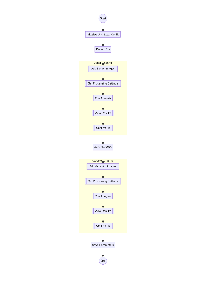
Flow of the bleed-through stage, from loading control images to saving the fitted coefficients.
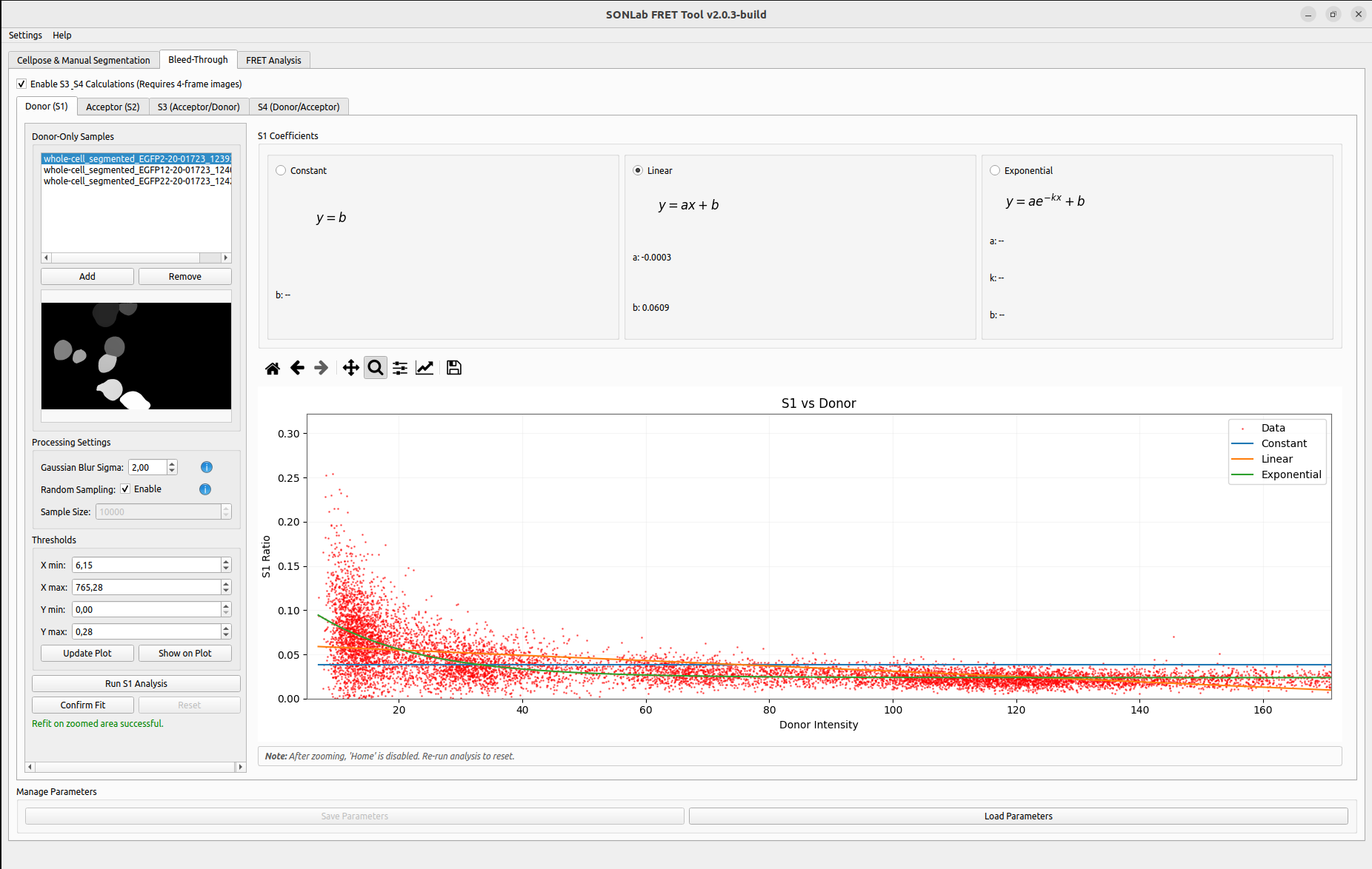 The Donor (S1) channel: control-image list and processing settings on the left, the coefficient/fit-model panel on top, and the S1-vs-Donor scatter plot with the Constant/Linear/Exponential fits below.
The tab contains up to four channel sub-tabs:
| Sub-tab | Coefficient | Control sample | Required |
|---|---|---|---|
| Donor (S1) | Donor → FRET bleed-through | donor-only | Always |
| Acceptor (S2) | Acceptor → FRET bleed-through | acceptor-only | Always |
| S3 (Acceptor/Donor) | Acceptor-channel cross term | donor-only (4-frame) | Optional |
| S4 (Donor/Acceptor) | Donor-channel cross term | acceptor-only (4-frame) | Optional |
S3 and S4 are enabled with the Enable S3 & S4 Calculations (Requires 4-frame images) checkbox and are only meaningful when your images contain four frames (mask, FRET, Donor, Acceptor).
- Select a channel sub-tab (start with Donor (S1)).
- Add the appropriate single-label control images.
- Configure the processing settings.
- Run the analysis to compute the bleed-through ratio and fit it.
- Choose the fitting model and confirm the fit.
- Repeat for the Acceptor (S2) channel (and S3/S4 if enabled).
- Save the parameters for reuse.
- Click Add, or drag & drop
.tif/.tifffiles onto the list. - A preview of the selected image's first frame is shown.
- Use Remove to drop images. When the list becomes empty, the preview, plot, and coefficients are cleared automatically.
Use donor-only samples for S1/S3 and acceptor-only samples for S2/S4. These should be the segmented stacks produced in the Segmentation tab (or sent there via Send to Donor / Send to Acceptor).
| Setting | Default | Description |
|---|---|---|
| Gaussian Blur Sigma | 2.0 |
Standard deviation of the Gaussian smoothing kernel applied before computing ratios; reduces pixel noise. |
| Random Sampling ▸ Enable | off | When enabled, the fit uses a random subset of pixels instead of all of them — much faster on large datasets. |
| Sample Size | 10000 |
Number of pixels to sample when Random Sampling is enabled. |
- Click Run Analysis for the channel.
- The tool processes the images (inside the segmentation mask only) and shows a scatter plot of the bleed-through ratio versus intensity, together with the fitted curve(s).
- Review the fit visually. If the relationship is concentrated in one region, use the plot toolbar's zoom to focus, or restrict the data with the threshold controls (below) and click Update Plot.
Note: after zooming, the toolbar's Home button is disabled. Re-run the analysis (or use the threshold Update Plot) to reset the view.
The Thresholds panel restricts which data points are used for the fit:
- X min / X max — intensity range.
- Y min / Y max — ratio range (0–1).
- Update Plot — re-fits using only the points inside the thresholds.
- Show on Plot — draws the threshold lines on the scatter plot.
This is useful for excluding saturated pixels or low-signal noise before fitting.
Three models are available; select one with its radio button. The fitted coefficients are displayed for each.
| Model | Equation | When to use |
|---|---|---|
| Constant | y = b |
Bleed-through is essentially intensity-independent. |
| Linear | y = a·x + b |
Bleed-through varies linearly with intensity. |
| Exponential | y = a·e^(−k·x) + b |
Bleed-through changes non-linearly with intensity. The curve decays by default, so a growing relationship yields a negative k. |
When satisfied, click Confirm Fit to lock the coefficients for this channel so they can be used in FRET calculations. Reset unlocks the controls for a new analysis or refit.
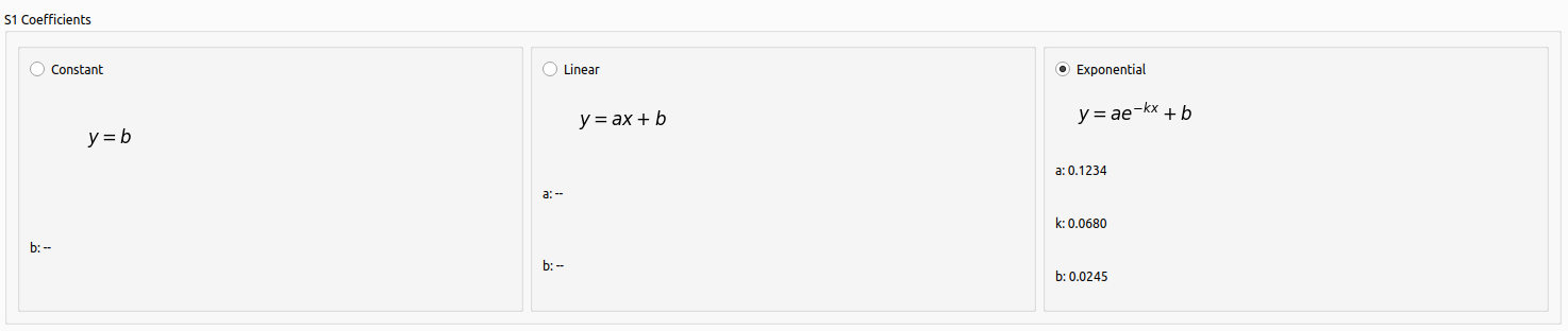 The coefficient panel: Constant (
y = b), Linear (y = ax + b), and Exponential (y = ae^(−kx) + b). Here Exponential is selected and its fitted coefficients (a, k, b) are shown.
In the Manage Parameters panel:
-
Save Parameters writes the model type and coefficients of all channels to
bt_params.jsonin the default location. It also writes a copy into each input image directory so the parameters stay alongside the data they describe; if a file already exists there, you are asked whether to overwrite it. - Load Parameters restores a previously saved file. On startup the tool offers to reload the last session's parameters automatically.
Loading parameters while an analysis is already on screen re-draws the plot from the saved coefficients (it does not silently re-fit), so confirmed values are preserved exactly.
For each channel you get:
- A scatter plot of the data with the selected fit overlaid.
- The calculated coefficients for each model.
- Interactive zoom/pan controls.
- Status messages indicating fit availability and quality.
The confirmed coefficients flow into the FRET Analysis tab. See Workflows and Data Flow.
| Symptom | Try this |
|---|---|
| Poor fit | Try a different model, or adjust the Gaussian Blur Sigma. |
| Slow performance | Enable Random Sampling with a smaller Sample Size. |
| No data points | Confirm the images are single-label controls in the correct channel and contain a segmentation mask. |
| Fit/plot not updating | Click the plot toolbar's Home, use threshold Update Plot, or re-run the analysis. |
| "S3 requires 4-frame images" | Provide 4-frame stacks (mask, FRET, Donor, Acceptor) when S3/S4 is enabled. |