Data view

Data view

The data view is the logic analyzer of openSciLab: it captures with a device, shows captures, files and test signals, and analyses, decodes and edits them. This page covers capturing (settings, triggers, streams, analog channels, state mode), finding your way around a capture and the analysis tools. Protocol decoders have a page of their own: Protocol decoders.

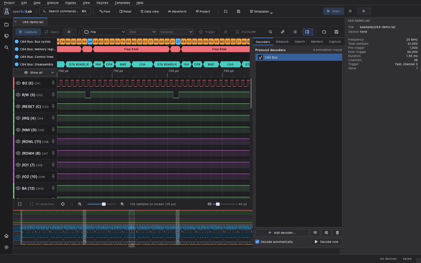
Shortcuts are written with Ctrl; on macOS that is Cmd. Help → Keyboard shortcuts... lists every key and gesture and can be searched.

Opening a data view

• From a device: Capture... in the header of its device card (see Devices), or Devices → Show data → (device).
• From a template: Templates → Start a project → Logic Analyzer opens a data view with the connected device. With several devices connected it asks which one; without one it shows the device list.
• Empty: Project → New → Data view, or Data view in the header. Choose the device in the tool bar.
• A file: Project → Open file... (Ctrl+O) or Open in the tool bar opens .lac, .lac.gz and .sr captures (see Files).

A data view without data says so (No data) and offers Devices... (or Device card...), Open capture... and Test signals....

Data views of a flow's data (Run data, a view.scope node, see Flows) show, search, measure, decode and save, but have no capture tool bar, no device and no Open.

The parts of the window

Part	What it holds
Tool bar	Capture, Again, Stop, the device, rate, length and trigger, Settings..., Profiles, the state of the device; Search, Measure, Listing, Panels, Open, Save
Annotation rows	the output of the protocol decoders, above the time axis
Time axis (ruler)	time from the trigger; selection, cursors, markers, the sample menu
Buses	buses and groups, below the time axis
Channels	pinned channels on top, then the others; analog channels as tracks below them
View bar	Fit, Fit selection, Trigger, zoom, samples on screen, height of the channels
Overview	the whole capture in small (Display → Capture overview)
Analysis panels (right)	tabs Decoders, Measure, Search, Markers, Capture (Ctrl+1)
Listing (bottom)	every change of the channels, or the decoder output (Ctrl+2)

While a data view is the active document, the menu bar has its menus Data, Analyze and Display, and the Project menu has New capture... and Export. The tool bar adapts to the width: less important entries show only their icon or move under More. A right click on the tool bar gives Customize toolbar... and Reset toolbar. The analysis panels and the listing can be moved, closed and opened again.

The Capture tab has two parts: the figures of the capture on screen (rate, samples before and after the trigger, duration, channels, trigger) and the settings of the next capture with a table of the device's channels (Channel, Pin, Name, Captured).

Capturing

A first capture without hardware:

1. On the start page, Try a simulator → Simulation: Pico (or any other simulator). Its device card opens.
2. Press Capture... in the card's header. A data view for the device opens.
3. Choose the rate and the length in the tool bar.
4. Press Capture (F5, also Capture in the header).

The state in the tool bar says what the device does: Ready, Armed, waiting for the trigger, Receiving n %, Last capture: n samples or Capture failed: .... A failed capture shows a banner above the waveform (with Device card) instead of a dialog.

• Again (Ctrl+R, Data → Capture again) captures with the settings of the last capture.
• Stop (Shift+F5, Data → Stop capture) ends a running capture. A stopped stream keeps what arrived.
• The device chooser in the tool bar switches to another connected device (Connect a device... opens the device list).
• A new capture never replaces data you have changed: it opens in another data view.
• Data → Use these channel names for the next capture gives the names you typed in the data view to the device.

Quick settings

The tool bar holds the most used settings: the sample rate, the length (samples and their duration, e.g. 1 M · 10 ms) and the trigger button, which names the trigger (Edge ↑ CH1, No trigger, Sequence, 2 stages, ...) and opens all settings. They are stored per kind of device and are the same settings the dialog shows.

Capture settings

Settings... opens all settings of the next capture on three pages. The line below the pages says what the capture will be; a problem is explained in the dialog and its page is marked. Start capture captures, Use settings only keeps the settings (the channel names appear in the device card at once), Reset restores the defaults. The dialog only offers what the device can do.

• Sampling: Frequency (the Jitter chip shows how far the real rate is from the one asked for; rates that divide the device's clock exactly show 0 %), Pre-trigger samples, Post-trigger samples (Max fills the memory) and a line with the total length. Devices with several modes have Acquisition (Buffer (device memory) or Stream (over USB)), Until stopped and Record to disk (see Streams). Some devices have a Threshold for the input voltage, some an External clock (see State mode).
• Channels: a check box, a colour and a name per channel (CH1, CH2, ...); All, None and Inv per row of eight, Select all and Clear for all. Enter in a name moves to the next one. Name your channels: decoders find their inputs by name. Fewer channels usually allow longer captures. Devices with analog inputs list them under Analog:.
• Trigger:
  • Edge: start when a channel changes level - the Channel (or External trigger on devices with a trigger input), Falling edge, Blast mode (the highest rate of the device, without pre-trigger samples) and Burst mode: (re-arm and capture several bursts, optionally Measure delays between bursts).
  • Pattern: start when channels match a bit pattern - First channel and Pattern (1011, first channel first), Fast matching (max. 5 bits). A pattern covers consecutive trigger inputs of one board; on a Pico channels 1-21 or 22-24.
  • None: start capturing at once (devices that can).
  • Sequence: stages of patterns, edges, pulse widths and gaps (below).
  • Evaluate the trigger in the application (on a stream, at the stream rates) (below).

Trigger sequences

A sequence waits for up to 8 stages. Each stage waits for an Edge, a Pattern (from a channel, X for any level, e.g. 10X1), a Pulse width (high, low or either, at least and/or at most a time) or a Gap (no edge for) a time, a number of Times, optionally within a time after the previous stage - otherwise the sequence starts over. The capture triggers when the last stage completes. Times are typed with units: 1 µs, 2 us, 10 ms.

Devices that evaluate sequences themselves (the Pico firmware, up to a highest rate it reports) do so in the device. Otherwise the application evaluates them on a stream (next section); the dialog ticks that for you and says when a sequence does not fit the device.

Software trigger

Evaluate the trigger in the application lets the device stream without a trigger while openSciLab looks for the trigger in the samples and keeps the samples before (up to half of the stream's length) and after it. It works with every kind of trigger, also on devices whose streams have none of their own (the Pico boards), but only at the stream rates.

Streams

With Stream (over USB) the device sends its samples while it captures. The data view shows them live and follows the newest samples; Roll in the view bar holds the view still (zoom and scroll back at any time). The status bar counts the samples and any lost ones.

• Until stopped: the stream runs until Stop and keeps only its latest samples, as many as Keep last samples: says.
• Record to disk: the stream goes into memory-mapped files instead of memory, limited by the free disk space (the dialog shows how much it needs). Decoders then run only on request (Decode now). The files are deleted with the capture; save it as .lac to keep it.
• A Pico board streams over USB only (not WiFi, not as a multi device set), starts at once without a trigger (unless the application evaluates it), and USB full speed limits it to about 800 kHz with 8 channels, 400 kHz with 16 and 200 kHz with 24 channels. The buffer mode keeps the high rates.

If a stream cannot keep up, the capture ends early with what arrived and says so in a banner; see Troubleshooting.

Analog channels

Devices with analog inputs (Arduino A0-A5, Pico GP26-GP28, the simulated DAQ and oscilloscope) capture them together with the logic channels: tick them under Analog: on the Channels page. They are drawn as tracks below the logic channels on the same time axis, with their value at the pointer and at the cursors; the Measure tab adds minimum, maximum, mean, RMS and peak to peak. A right click on a track offers Digital channel from a threshold... (with hysteresis), Hide, Taller tracks and Shorter tracks. The overview shows analog channels as an envelope.

Large captures of an oscilloscope arrive piece by piece: the part on screen comes first, missing parts are hatched, and saving, exporting and decoding wait until all of it is there.

State mode

External clock: on the Sampling page (devices with a state mode, e.g. the Pico boards and the simulated analyzer) takes one sample on every rising or falling edge of a clock channel instead of at a fixed rate: the device under test clocks the analyzer. The time of every state is kept. The data view shows the states one after the other on a numbered axis; Real time in the view bar shows them on their real time. The example Basics → State mode shows it in a flow.

To resample a capture you already have on a clock, use Analyze → State analysis (clocked)... (see Analysis).

Test signals and composed captures

• Data → Test signals... computes a counter, a walking one or Protocols (UART, SPI, I2C) carrying the text "openSciLab" on this computer; Add UART, SPI and I2C decoders for the channels adds matching decoders. A Pico board can generate the same signals itself (Test signals of the board... on its device card).
• Project → New capture... composes a capture: choose channels and timing, then describe each channel in the Signal Description Language ($0;h10;l10; - start low, 10 samples high, 10 low; the editor explains the rest).

Moving around

Action	Input
Zoom	mouse wheel over the waveform, ruler, buses, analog tracks or annotations (Shift: bigger steps); + / -; pinch on a trackpad; Ctrl + two-finger swipe up/down
Show the whole capture	Ctrl+0, Fit, two-finger double tap
Show the selected samples	Ctrl+E, Fit selection
Go to the trigger	Ctrl+T, Trigger
Scroll sideways	Ctrl + wheel, horizontal wheel, two-finger swipe, drag the waveform, ← → (10 %), the scroll bar, click or drag in the overview
Page / one sample	Ctrl+↑ Ctrl+↓ / Shift+← Shift+→
Scroll through the channels	swipe up/down on a trackpad, the scroll bar
Height of the channels	Alt + wheel, Ctrl+Shift+↑ / ↓, Ctrl+Shift+0 (default), the slider in the view bar

Settings → Navigation swaps what the wheel does (zoom or move) and the zoom direction. Keys without Ctrl (arrows, +, -, A, B, M) only act while the data view has the focus. Resting the pointer on a channel shows the sample, its level, the length of the pulse and the frequency it suggests.

Channels

• Rename: double-click the name (or right-click → Rename...).
• Colour: click the coloured strip left of the name (or Colour...).
• Hide: the eye button; the button above the names says how many are hidden and shows them again, one by one or all (Display → Show all channels).
• Pin: the pin button keeps a channel at the top while the others scroll (Display → Unpin all channels).
• Order: drag a channel by its name, or Move up / Move down.

Names, colours, order, hidden and pinned channels are saved with the capture.

Selection, cursors and markers

• Select samples: drag in the ruler; Shift + click extends the selection. It shows over every track. A click without dragging sets (or removes) a marker line.
• Cursors A and B: drag them on the ruler, press A or B with the pointer over the waveform, or right-click the ruler: Place cursor A here, Place cursor B here, Cursors to the selection.
• Named markers: M at the pointer, or Add marker here in the ruler's menu. The Markers tab lists markers and regions (double-click to go there) with Add marker, Edit... and Remove.
• Regions: select samples, right-click → Create region from selection..., give it a name and a colour. Edit... on the Markers tab renames and recolours it.
• Everything set on a device while a capture runs (a pin, a pulse) becomes a marker in the capture; ≈ marks a time taken from the computer's clock.

Analysis

Measure

Measure (Ctrl+Shift+M) shows:

• Cursors: A, B, Δt (B − A), 1 / Δt, Δ samples, the level of every channel at A and B and the edges between them; Place in view, Zoom to A–B, Clear.
• Statistics of every channel Between the cursors, in the Visible part or the Whole capture: frequency, duty cycle, shortest and longest high and low pulses, edges.
• Analog: value at A and B, minimum, maximum, mean, RMS, peak to peak.
• Setup and hold: of a data channel around the rising or falling edges of a clock channel.

Measure selection... in the ruler's menu shows pulse statistics of every channel over the selected samples.

Search

Search (Ctrl+F, Analyze → Find...) finds an Edge, a Pattern (10X1 from a first channel), a Pulse width (at least / at most), a Gap (no edge for) a time, a Bus value (==, !=, <, <=, >, >=, in; 0x1F, 31, 0b11111 or a symbol) or Decoder output (text, optionally Regular expression and Match case). Find all marks every match in the waveform and lists them; F3 / Shift+F3 go to the next / previous one.

Buses and groups

Analyze → New bus or group... shows several channels as one value. Give it a Name, choose Show values as (Hexadecimal, Decimal, Signed decimal, Binary, ASCII), tick the channels (the topmost is bit 0; Reverse swaps the order) and optionally a symbol table that shows names instead of values (IDLE = 0x00, $D020 NAME, CSV, or Load symbol file...). Buses appear below the time axis; double-click one, or right-click for Edit bus..., Remove bus and New bus.... They are saved with the capture.

Listing

Listing (Ctrl+2) shows a table below the waveform: Changes of channels and buses (a row per change, with time, sample and the value of every channel and bus) or the Decoder output. With Follow the view it scrolls along with the waveform; a click on a row marks its sample in the waveform.

More in the Analyze menu

• Charts and histograms... - a bus value over time, and histograms of high pulses, low pulses and periods of a channel or of the values of a bus, over the whole capture, the visible part or between the cursors.
• Compare with a reference... - compares every channel with the same channel of a reference capture file, finds the offset (Find automatically), ignores jitter up to a Tolerance, and marks the differences as search matches (F3 jumps to the next) or Mark as regions. Two captures selected in the Data part of the sidebar can be compared with a right click as well.
• State analysis (clocked)... - resamples the capture on the edges of a clock channel, like an analyzer clocked by the device under test, optionally Only when qualifier channels match (CH3=0 CH4=1). It suggests the edge and Sample offset at which the other lines are stable. Back to the timing capture returns. Decoders that follow the clock themselves, such as the C64 bus, work on the timing capture.
• Play as signal... - the digital channels as a pattern, or an analog channel as an arbitrary waveform, for a generator output (between the cursors if both are set).

Multi device sets: Data → Align boards aligns the boards of a capture again, see Multi-device sets.

Editing samples

Select samples in the ruler, then use the Data menu or right-click the ruler: Cut samples (Ctrl+X), Copy samples (Ctrl+C), Paste samples (Ctrl+V), Delete samples (Delete), Insert samples... (described in the Signal Description Language) and Shift channels..., which moves the samples of chosen channels left (earlier) or right (later) by a number of samples, filling with low, high or what was pushed out at the other end - useful for a probe that was one sample late.

Every change of the data - samples, channels, markers, regions, buses - can be undone with Edit → Undo (Ctrl+Z) and redone with Edit → Redo.

Profiles

A profile stores capture settings (channels with names and colours, rate, length, trigger, bursts) together with the protocol decoders, so a setup comes back with one click. Profiles in the tool bar (with a device chosen; also in the header of the device card) has:

• Save current settings as profile... - the settings of the shown capture (or the last ones of the device) and the decoders of this data view.
• My profiles - each with Load, Edit... (name, notes, capture settings, decoders) and Delete....
• Standard profiles - ready-made setups with the wiring in their notes: UART (9600 and 115200 baud), MIDI, DMX512, LIN, I²C (100 and 400 kHz), SPI mode 0, 1-Wire, CAN 500 kbit/s, PWM and servo, WS2812, I²S, an 8 bit parallel bus, SWD, JTAG, IR (NEC), USB low and full speed, and the C64 expansion port.
• Open the profiles folder, Import profiles..., Export profiles....

Loading a profile applies its decoders to the data view of the device - or, when none is open, to the next one (loading opens no view); its capture settings apply to the next capture of this device, fitted to what the device can do (the status bar says what changed). A profile that needs channels the device does not have is shown but cannot be loaded, with the reason. Where profiles are stored: Files.

Saving

Project → Save (Ctrl+S) writes the capture to its .lac file, or asks for a name; Save as... also offers compressed .lac.gz and the form of the original LogicAnalyzer software. Project → Export writes CSV, VCD, sigrok sessions for PulseView and the decoder output. The decoders themselves are not part of a capture file - keep them in a profile. Details: Files.