Getting started

Getting started

This page shows around the window and the start page, walks through a first measurement with a simulator (no hardware needed) and with a real board, and explains projects and the settings.

Shortcuts are written with Ctrl; on macOS that is Cmd.

The window

Part	Where	What it holds
Header	top	the logo, Search commands... (Ctrl+K), buttons for a new Flow, Panel, Data view, Waveform and Project, Open, Save, Templates, and Start / Pause / Stop for the active document
Activity bar	far left	the sidebar sections Project (Ctrl+Shift+E), Devices (Ctrl+Shift+D) and Search (Ctrl+Shift+F); at the bottom Start (the start page) and Settings
Sidebar	left	Project: open documents, the files of the project, its data, recent files. Devices: Connected devices and Available ones, with the buttons Hardware... and Refresh. Search: commands, documents and files
Documents	middle	data views, flows, panels, waveforms, device cards, in tabs with their close button on the left
Node palette	beside a flow	the nodes to drag into the flow (View → Node palette, Ctrl+Shift+N)
Inspector	right	the properties of what is selected: a node, a panel widget, a device (Ctrl+Alt+I)
Console	bottom	Problems, Execution (what a flow does), Log and a Python console (Ctrl+J)
Status bar	bottom	Real time or Virtual time of the active flow, the number of devices, unsaved documents, problems

Clicking the icon of the section that is shown hides the sidebar (Ctrl+B too). A right click on the activity bar shows, hides and orders its entries and can put names under the icons. The parts of a sidebar section open and close with a click on their header. Tool bars give way when the window is narrow (the rest moves into a ⋯ menu); a right click on a bar offers Customize toolbar....

A document tab has a menu on its right click: Close others, Split right, Split down, Open in a new window. View → Layout → Save layout as... keeps an arrangement, Reset layout restores the default one.

Menus: Project (new, open, save, close, settings), Edit (undo, redo, command palette), the menus of the active document (Data, Analyze and Display for a data view, Flow for a flow), View, Devices (connect, device cards, disconnect, connected hardware, simulated faults), Templates and Help. Help → Keyboard shortcuts... lists every shortcut and can be searched; Help → Online documentation opens this wiki.

The command palette (Ctrl+K or the search field in the header) finds every command, open document, recent file and template by a few letters of its name.

The start page

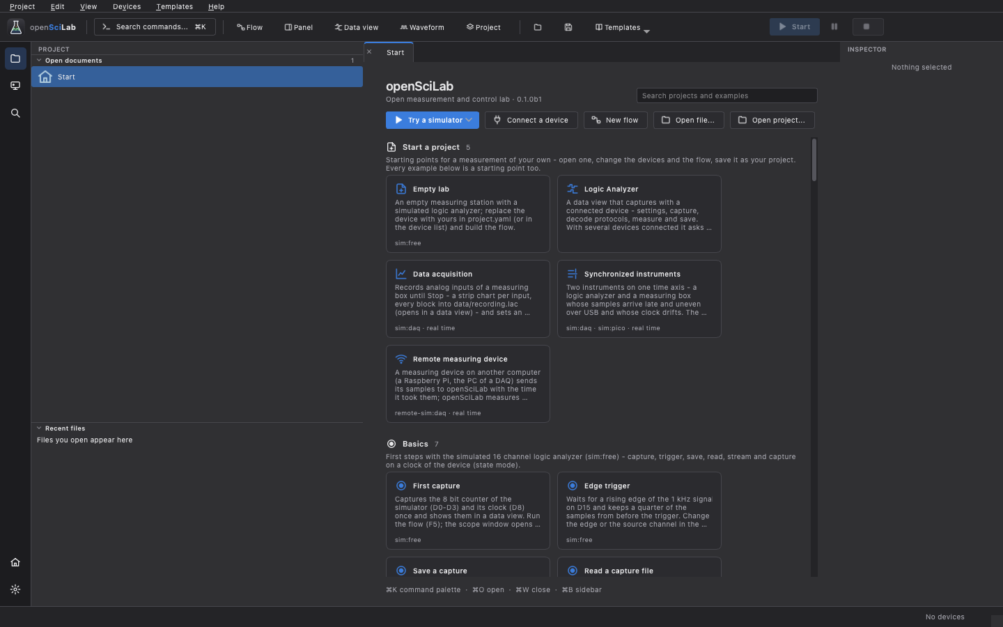
On the first start openSciLab shows the start page, with an empty flow beside it; when documents were saved in the last session, it opens them again (see Settings). The start page comes back with Start at the bottom of the activity bar, or Project → New project....

• Try a simulator opens a menu of the simulated devices (Simulation: Arduino Uno, Simulation: Pico, Simulation: USB DAQ, Simulation: DHO924S, …). The chosen one is connected and its device card opens. See Simulators.
• Connect a device opens the dialog Connect a device: boards found on USB (Detected), entries for devices in the network (Add by hand) and the Simulators.
• New flow, Open file..., Open project....
• Below them, every project of the example library is a tile, sorted by category, with a search field (Search projects and examples). A click opens the project as a temporary copy (see Projects); every one of them runs with simulators.
• On the right, the recent files and projects.

My templates comes first once you saved a project as a template of your own (see Projects). The next category, Start a project, holds the plain starting points:

Template	What it is
Empty lab	an empty flow with a simulated logic analyzer (sim:free), to build your own
Logic Analyzer	a data view that captures with the connected device; asks which one when several are connected, shows the device list when none is
Data acquisition	records the analog inputs of a measuring box until Stop, sets an analog output from a panel
Synchronized instruments	a logic analyzer and a measuring box on one time axis, aligned by a sync signal
Remote measuring device	a device on another computer, with the script to run there

The other categories (Basics, Digital I/O, Analog, Protocols, Measurement, Signal generation, Control, Data and reports, Panels, Python, Advanced, Remote devices, Time) are small examples that explain themselves; each one is a starting point too. The Templates menu has the same projects, one sub-menu per category, and All templates (start page). The full list is in examples/library/README.md.

A first measurement with a simulator

No hardware needed: the simulated logic analyzer Simulation: free has 16 channels with test signals - an 8 bit counter on D0-D7 with its clock on D8, UART on D9, SPI on D10-D12, I²C on D13-D14 and 1 kHz on D15.

In the data view (the logic analyzer)

1. On the start page, choose Try a simulator → Simulation: free. Its device card opens, with the tabs Pins, Signals, Events, Timing and Details.
2. Press Capture... in the header of the card. A data view opens that captures with the simulator.
3. The tool bar of the data view shows the settings of the next capture: rate, length and the trigger button (here No trigger); Settings... opens all of them (channels, names, trigger, acquisition). The defaults - 100 MHz, 1 M samples (10 ms) - are fine.
4. Press Capture (F5). The state next to the settings says what happens (Armed, waiting for the trigger, Receiving …), then the waveform appears. The channels are numbered from 1, so D0 is Channel 1 and D9 is Channel 10.
5. Decode the UART: in the panels on the right (Panels in the tool bar, Ctrl+1, if they are hidden), tab Decoders → Add decoder... → search UART → Add decoder. In its settings choose RX = 10: Channel 10; the baud rate is already 115200. Apply: the annotation rows of the decoder show the bytes of the text openSciLab.

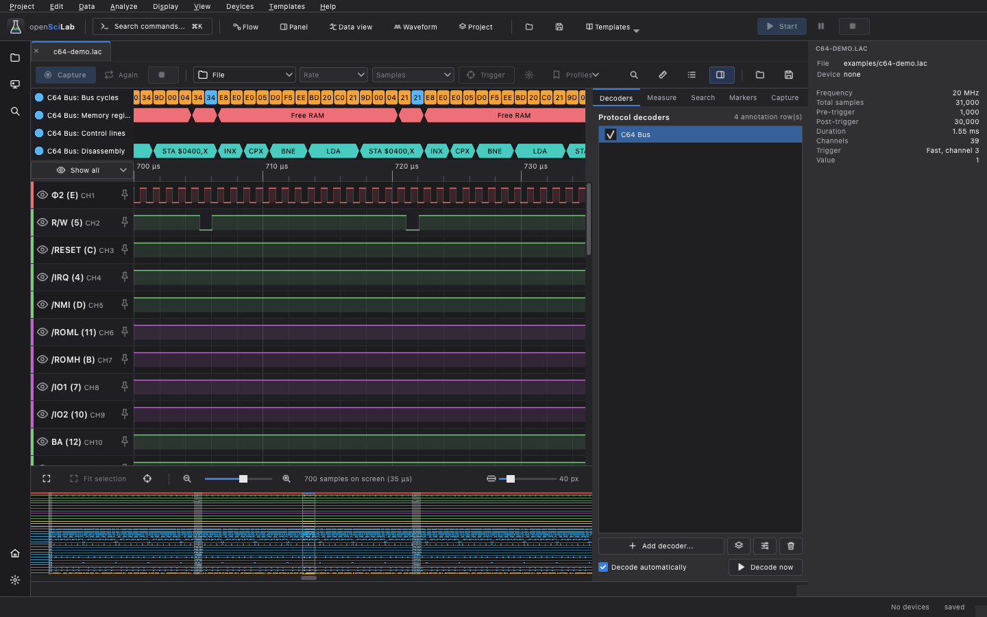
Zoom with the mouse wheel, fit the whole capture with Ctrl+0, and save it with Ctrl+S (.lac, .sr, …). Everything the data view can do is on the page Data view, the decoders on Protocol decoders.

To try something else, open the Signals tab of the device card, choose for example UART in Simulates, type your own text and press Apply; the next capture shows it.

In a flow

1. Templates → Basics → First capture (or its tile on the start page). A flow opens: a device, a capture of five channels at 4 MHz, and a scope.
2. Press Run in the tool bar of the flow (or Start in the header, F5). The scope opens a view with the capture; the nodes show their data.
3. Tick Fast (virtual time) in the flow's tool bar to run it as fast as possible and with the same result every time.

What flows are and how to build them: Flows and Nodes.

A first measurement with a real board

The inputs of the boards tolerate 3.3 V only. A 5 V signal needs a level shifter or a divider.

1. Firmware. A new Raspberry Pi Pico needs the openSciLab Pico firmware: hold its BOOTSEL button while plugging it in, open Devices → Connected hardware (or Hardware... below the device list) and press Install firmware in its row. The application picks the right image, writes it and connects the board again. Details and other boards: Firmware.
2. Connect. The board appears in the sidebar under Devices → Available as openSciLab Pico on and its port. Double-click it (or use Connect a device on the start page). Its device card opens.
3. Wire. Connect GND of the board to GND of your circuit and the signal to an input. On a Pico, channel 1 is GP2, channel 2 is GP3 and so on (GP2-GP22, then GP26-GP28); the Pins tab of the card shows the channel of every pin.
4. Capture. Capture... on the card opens the data view, as with the simulator. Set the rate (at least four times the fastest signal), the length and a trigger (Settings...), then Capture (F5).

Once a board is connected, the template Logic Analyzer opens a data view that captures with it directly. Arduino boards, DSLogic analyzers, oscilloscopes and devices in the network are described on Devices.

Projects

A project is a folder with everything of one measurement setup:

my-lab/
├── project.yaml     the project: name, devices, simulation wiring, files to open
├── flows/           flows (*.flow.yaml, Python flows)
├── panels/          panels (*.panel.yaml)
├── nodes/           own node types (Python)
├── waveforms/       waveforms (*.wave.yaml, *.sdl)
├── data/            what the flows write: captures, tables, logs, reports
└── tests/           flow tests against the simulator

project.yaml names the devices every flow of the project can use, so a flow can be moved from a simulator to the real device by changing one line:

project: My lab
devices:
  la: sim:free          # later: pico:/dev/ttyACM0 or pico:COM5
open: [flows/main.flow.yaml]

• New project: open a template (start page, Templates, or Project → New project...). It opens as a temporary project, a copy in a temporary folder, so the library stays as it is.
• Saving: the first Save (Ctrl+S) of a document of a temporary project, or Project → Save project as..., asks for a folder name and copies the whole project there (by default into ~/Documents/openSciLab). Closing the last document of a temporary project that was not saved asks Save project... or Discard.
• Opening: Project → Open project... (Ctrl+Shift+O) takes a folder with a project.yaml; Project → Open recent lists recent projects and files.
• Your own templates: Project → Save project as template... (also at the top of the Templates menu) keeps the project of the active document as a template: a name, a description for its tile, and a copy of its flows, panels, nodes, waveforms and devices - not the captures and results in its data folder; the documents open at that moment open again with it. Changed documents of the project are saved first. Your templates come first, as My templates, on the start page and in the Templates menu; a new project from one is a temporary copy like any other. Delete one with a right click on its tile, or Templates → My templates → Delete. They are kept in the folder templates of the settings directory (see Files).
• The sidebar section Project lists the flows and panels of the project and, under Data, the files in its data/ folder; a double-click opens one, a right click on two selected captures offers Compare the two captures.

A flow that does not belong to a project writes its files next to the flow file, or into a temporary folder while it is not saved.

Settings

Project → Settings... (Ctrl+,; on macOS openSciLab → Settings..., Cmd+,), or Settings at the bottom of the activity bar.

Page	Settings
Appearance	Theme: Dark (default), Light or Like the system - applies after a restart, which openSciLab offers (Restart now). Text size: 10 px by default; 12 px gives the roomier spacing of earlier versions. The waveform stays dark in both themes
Startup	Show the start page; Open the saved documents of the last session again (on by default; unsaved documents never come back); Connect the devices of the last session again (off by default)
Navigation	what the Mouse wheel does in the flow graph and the waveform: Zooms or Moves (with Ctrl/Cmd the other); Turn the zoom direction around
Data	the Folder for new projects and save dialogs without a project; how many Recent entries are kept
Devices	Look for devices every … seconds; List the simulators with the devices; Read devices on USB in a process of their own (on by default); Read devices with a higher priority
Remote devices	accept devices on other computers, port and token; see Remote devices
Time	what this computer's clock follows (NTP, PTP), measured latencies; see Time and synchronization

Defaults resets every setting. The settings are stored in preferences.json in the settings directory (see Installation); the environment variable OPENSCILAB_THEME=light or dark overrides the theme for one start.