Flows

Flows

A flow is a measurement program drawn as a graph: nodes that capture, measure, decide, generate, store and show, connected by wires. This page covers the flow editor, running and debugging a flow, the values that travel on the wires, the *.flow.yaml file and, briefly, flows written in Python.

What a flow is

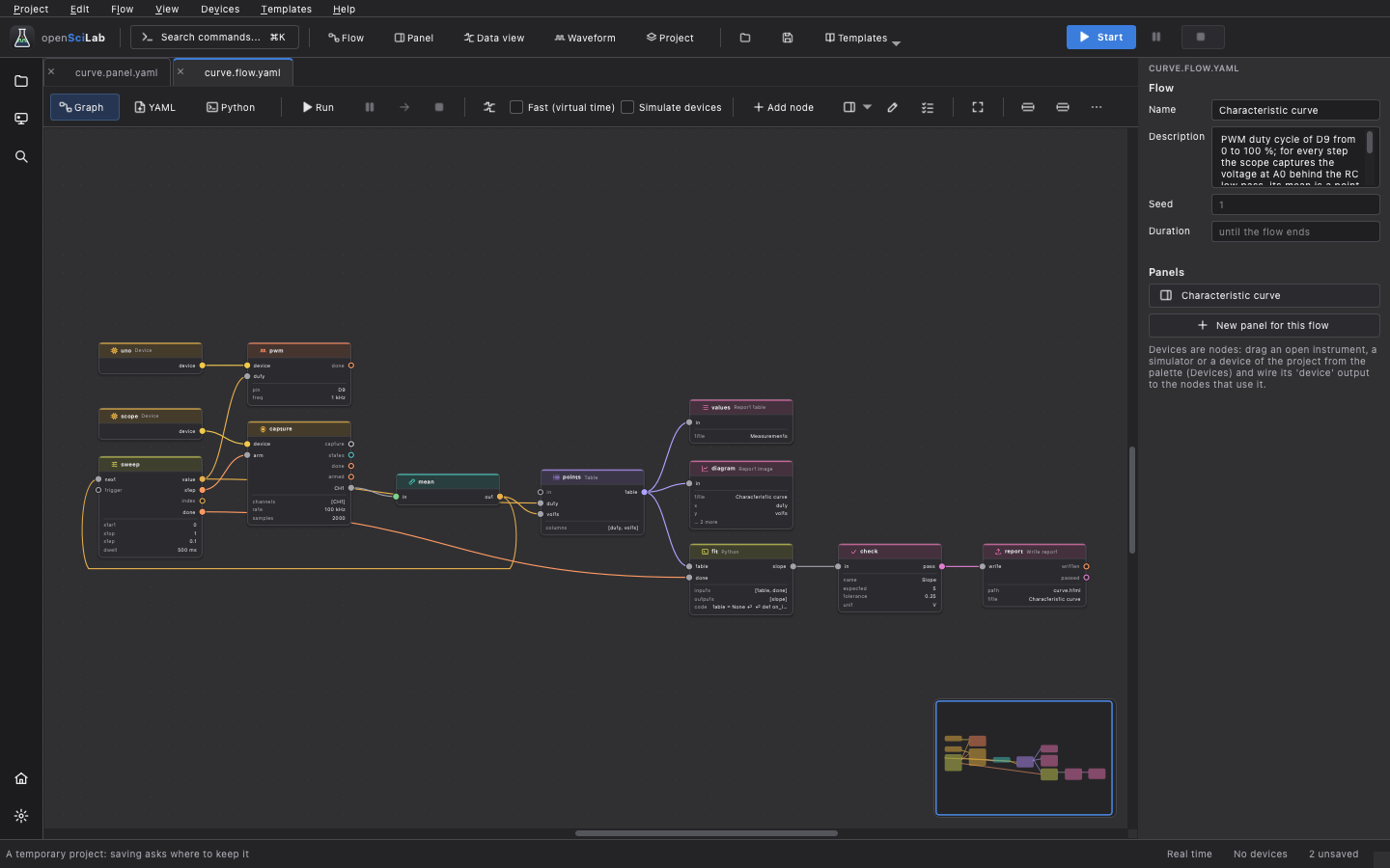
• Nodes do one thing each: capture with a device, measure a frequency, compare a value, write a file, show a chart. Nodes gives an overview of all families.
• Wires carry values from an output (right side of a node) to an input (left side). A node runs when values arrive; timers, sweeps and sequences run by themselves.
• Devices are nodes too. A device.instrument node stands for an instrument (a simulator such as sim:uno, a board such as pico:/dev/cu.usbmodem1, or an instrument already open in the device list). Its device output is wired to every node that uses it: capture, stream, monitor, GPIO, generator. Without an address the node is the project's device of the same name.
• A flow is saved as *.flow.yaml. The same flow can also be written as a Python script.

The quickest way to a working flow is an example: the projects in the Templates menu and on the start page are flows with simulated devices that run without hardware, and each one is a starting point for your own.

Making a flow

• New flow on the start page, Flow in the header, or Project → New → Flow (Ctrl+N).
• A flow that is not saved yet writes its files into a scratch folder; a saved flow writes next to its file; a flow of a project writes into the project's data/ folder (listed in the sidebar).
• Save asks for a *.flow.yaml name. In a project the dialog starts in its flows/ folder.

Shortcuts on this page say Ctrl; on macOS it is Cmd.

The editor

The flow document has three views, switched in its tool bar: Graph (the canvas), YAML (the file itself, editable) and Python (the same flow as a script, read only). Edits in any view change the same flow, with undo and redo for every step (Edit → Undo / Redo).

Adding nodes

• Node palette: beside a flow whose graph is shown (View → Node palette, Ctrl+Shift+N shows or hides it). Search with Search nodes, then drag a node onto the canvas or double-click it. Its first group, Devices, offers the open instruments, the project's devices and every simulator as ready device nodes. The Decoders group loads when you open or search it.
• On the canvas: press Tab, or just type a name; a search opens at the pointer.
• Tool bar: Add node…. A right click on the empty canvas offers Add node…, Comment, Paste and Select all.
• Device list: right-click an open device, Add to the flow.

A node that needs a device is wired at once when the flow has exactly one device node; adding the first device node wires the nodes that were waiting for one (the status bar says what was wired).

Wires

• Drag from a port to another port. While you drag, the ports the wire fits light up and the wire snaps to them (or to the right port of the node you drop it on).
• Drop a wire on the empty canvas: a list of the nodes it fits opens; the chosen node is placed there and wired.
• A wire that does not fit says why above the graph. If a conversion exists, the message has a button Insert … that puts the conversion node in between (see the table below).
• Right-click a wire: Insert a node… or Remove wire. Right-click a port: Add a connected node… or Disconnect all. Delete or Backspace removes the selected nodes and wires.
• Most inputs take one wire, and a new wire replaces the old one; inputs that collect (a log, a table, a counter, a scope) take several. A device wire fits only device inputs. Wires are coloured by the type of value they carry.

From	To	Conversion node
Analog	Digital	dsp.threshold (1 above a threshold, with hysteresis)
Digital	Analog	convert.to_analog (logic levels as volts)
Digital	Event	convert.edges
Analog	Scalar	measure.mean
Digital	Scalar	measure.duty
Scalar	Bool	control.compare (at or above 0.5)
Bool	Scalar	convert.to_scalar
Event	Table	data.table
Event	Scalar	control.counter
States	Digital	convert.state_bit
Capture	Digital, Analog	convert.channel

The inspector and the node editor window

Select a node and the inspector on the right shows its title, type and description, the problems found at it, its Name, every parameter (units in brackets, required ones marked with *), a Comment and the Breakpoint box. Changes apply at once. Where it can, the inspector offers what the wired device has: pins that can do what the node needs, channels to tick, generator outputs, the channels of the capture wired to a decoder, … to choose a file.

Double-click a node to open its parameters in a window of its own, with bigger text fields (mappings and long lists such as the states of a state machine are YAML, one entry a line; Ctrl+Return applies a big field). A double-click on the data a node shows opens that data in a view instead, and a double-click on a subflow opens the subflow.

With nothing selected, the inspector shows the flow: Name, Description, Seed (random numbers of simulators), Duration (empty: until the flow ends), the Panels that use the flow and New panel for this flow.

Values that do not fit (a word where a number belongs, a pin the device does not have, a channel the capture does not record) are warnings at the node, in the inspector and in the Problems tab of the console. Required inputs without a wire are marked. Check in the tool bar lists all problems.

Arranging, groups, comments, subflows

• Arrange (Ctrl+Shift+L) lays the selected nodes, or all, out along their wires, as one undo step. Auto-arrange (shown as Auto) does it again whenever nodes or wires are added or removed.
• Align left, Align top and Distribute are in the Flow menu; a right click on the tool bar (Customize toolbar…) puts them into the bar.
• Comment adds a note; Group draws a frame around the selected nodes. A group carries the nodes inside it when it is moved; groups and comments resize at their lower right corner.
• Make subflow (Flow menu, or the right-click menu with several nodes selected) moves the selected nodes into a subflow and puts one node in their place; the wires that crossed become its inputs and outputs. Double-click the subflow node (or Open subflow) to edit it in a tab of its own. Subflows are saved in the same file. Example: Templates → Control → Subflow.
• Cut, copy, paste, Duplicate (Ctrl+D) and Select all work with the wires between the nodes.

Moving around

Two fingers on a trackpad move the canvas, a pinch zooms. The mouse wheel zooms at the pointer (Ctrl+wheel moves sideways, Shift+wheel up and down; Settings → Navigation can swap zooming and moving). Space + drag or the middle button moves the canvas, + and - zoom. The Flow menu has Zoom in, Zoom out, Fit (Ctrl+0) and Actual size. The overview (minimap) in the lower right corner shows the whole flow, its nodes in the colours of their kinds; click or drag in it to move there.

Running a flow

Run (F5) in the flow's tool bar, or Start in the header, starts the flow; Pause, Step (F10) and Stop (Shift+F5) are beside it. The console opens on its Execution tab.

Setting	Meaning
Fast (virtual time) off	Real time: timers wait real seconds, devices run as they do. Needed for real hardware and remote devices.
Fast (virtual time) on	Virtual time: with simulators the flow runs as fast as possible, the clock jumps to the next thing that happens, and every run gives the same result.
Simulate devices	Every device node of the flow uses a simulator instead of its address.
Duration (inspector of the flow)	End the flow after this time (real or virtual), e.g. 10 s, 1 h.

The status bar shows whether the active flow runs in Real time or Virtual time. A flow ends when nothing can happen any more, after its duration, or with Stop. Also after Stop or an error, what it measured is written (the rows of a logger, recorded samples, the report). If a device is missing, the message above the graph offers Run with simulators. If the flow cannot start, the message says why and Show problems opens the list. Changes in the inspector while a flow runs apply to its next run.

While the flow runs, every node shows its state, wires show the latest value (a small sparkline for numbers), and nodes show their data below their parameters: a trace of the latest capture, the latest value, the rows of a table. View nodes (scope, strip chart, number, ...) open documents of their own.

Looking at the data of a run

• Run data in the tool bar shows all data of the run in one data view on one time axis: the channels of every capture, sampled signals, measurements as lines that step from value to value, checks as digital lines. It follows a running flow and the next run.
• Show data in a node's right-click menu (or a double-click on its data) opens the data of that node; a table opens as a table.
• Show data in the nodes and Clear run data are in the Flow menu.

Debugging: pause, step, breakpoints

• Pause holds the flow; Run turns into Continue.
• A breakpoint stops the flow before that node handles a value. Set it with the dot that appears on a node under the pointer, with Breakpoint in the node's right-click menu or with the Breakpoint box in the inspector.
• While paused, Step (F10) lets one node handle one value. Templates → Control → Timer and counter is a good flow to try this on.

Values and types

Every port has a type; a wire fits when both ends have the same type, or one of them is Any.

Type	What it carries
Digital	a logic signal: samples of one channel with their rate and time
Analog	sampled voltages (or another unit)
Scalar	one number with its unit, e.g. a frequency
Bool	true or false, e.g. the result of a check
Event	something that happened at a time, possibly with data (a tick, a decoded byte)
States	samples taken on the edges of a clock (state mode)
Capture	a whole capture: several channels, digital and analog
Table	rows and columns
Any	whatever arrives
Device	the connection from a device node to the nodes that use it

A capture or stream node also has an output per channel (capture.D8, stream.AI0), so a single channel can be wired straight into a measurement. Blocks of a stream arrive one after another; measurements work on each block. Parameters take quantities with units: 4 MHz, 1.2 ms, 3.3 V, 20 mA, 50 %. 5m is 5 milliseconds; minutes are 5 min.

Values wait at the inputs in the order they came; a node that is slow holds its senders back instead of losing values. If nodes wait for each other for ever, the flow ends with the error deadlock.

The flow file

flow: Counter
description: Captures the counter of the simulator and saves it.
settings:
  duration: 10 s
nodes:
  sim: {type: device.instrument, address: sim:free}
  cap: {type: device.capture, channels: [D0, D1, D8], rate: 4 MHz, samples: 20000,
        trigger: {edge: rising, source: D8}}
  scope: {type: view.scope, title: Counter}
  file: {type: data.file, path: counter.lac}
edges:
  - sim.device -> cap.device
  - cap.capture -> scope.in
  - cap.capture -> file.in

• Sections: flow (name), description, settings (seed, duration), inputs and outputs (of a subflow), nodes, edges, subflows.
• A node is its type and its parameters; at: [x, y] is its place on the canvas, comment its comment. An edge is node.output -> node.input.
• The file is read as YAML 1.2: only true and false are truth values (on, off, yes and no stay text, so a state machine may have a state off).
• The editor writes one tidy form, so files diff well; comments in hand-written files are not kept.

In the YAML view the editor completes section names, node types after type:, parameters that are not set yet, their values (choices, the pins and channels of the device) and the ports in edges. The list opens by itself or with Ctrl+Space; Enter or Tab takes a completion. YAML with an error stays as typed: leaving the view asks Keep editing or Discard the changes.

Flows in Python

The same flow as a script, with the DSL of openscilab.lab:

from openscilab.lab import flow, nodes as n

with flow("Counter") as f:
    sim = f.device("sim", "sim:free")
    cap = n.device.capture(sim, channels=["D0", "D1", "D8"], rate="4 MHz", samples=20000,
                           trigger=n.edge("D8"))
    cap.capture >> n.view.scope(title="Counter")
    cap.capture >> n.data.file(path="counter.lac")

result = f.run(fast=True)

n.<group>.<name>(...) adds a node, a.out >> b.in wires two ports. YAML and Python convert into each other unchanged. The application opens such a script as a graph; Save then writes a .flow.yaml and never overwrites the script. More in Scripting; an example is Templates → Python → Flow as a Python script.

See also

• Nodes – what each family of nodes is for, and nodes of your own
• Panels and reports – front panels for a flow, reports with checks
• Time and synchronization – when the samples of a flow were taken
• Scripting – openscilab run and the Python API
• docs/lab.md – the reference of flows, nodes, panels and projects