A first example setup

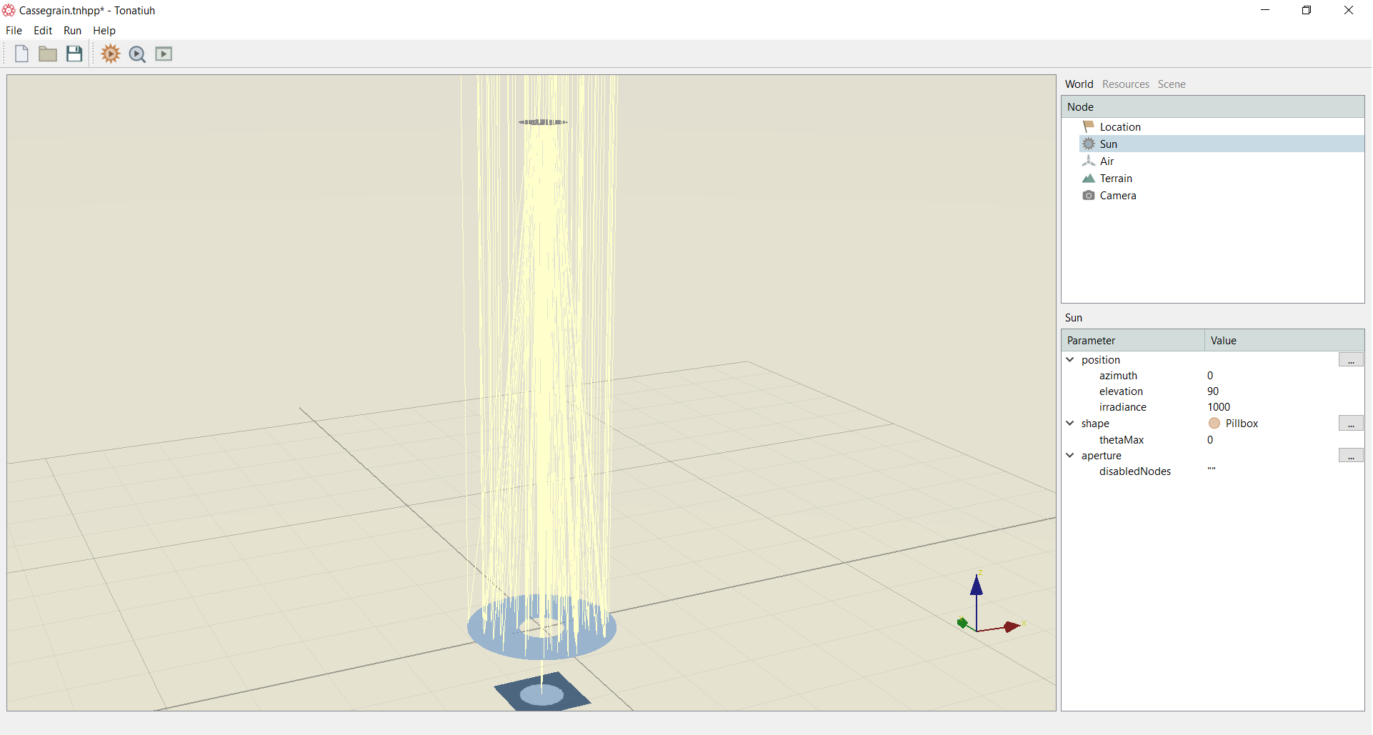
For illustrating how to step-by-step set-up and run a ray-tracing simulation, a Cassegrain reflector simulation as shown in Figure 1 is discussed in this page. The Cassegrain reflector is a combination of a primary concave mirror and a secondary convex mirror, often used in optical telescopes and radio antennas, the main characteristic being that the optical path folds back onto itself, relative to the optical system's primary mirror entrance aperture. The reflector is composed of three components, a primary mirror, a secondary mirror and a receiver.

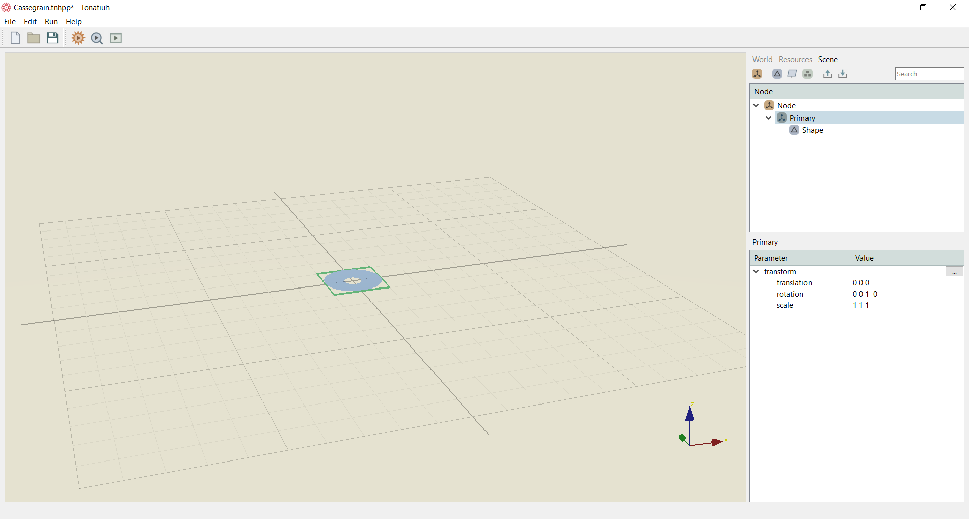
For creating the simulation scene, press the Scene tab on the vertical panel at the right of the screen. A Node is defined as a brown button with a cartesian coordinate system sign inside. A Shape is defined as a gray button with a triangle inside. To add the primary mirror, press the Node and then on the node add a Shape as shown in Figure 2. Rename the Node as Primary by double-clicking on the name. Clicking on the Primary node will enable the user to set the parameters of the node in the bottom panel. Here the translation, rotation and scale of the scene (if any) within the terrain grid can be set. For this primary mirror, we are keeping its location in the center of the grid, so no parameters should be changed here and must be kept as shown in Figure 2.

By pressing on the shape icon the related parameters will come up in the bottom panel. Here the user can set-up the parameters related to the shape and optics of the primary mirror as shown in Figure 3.

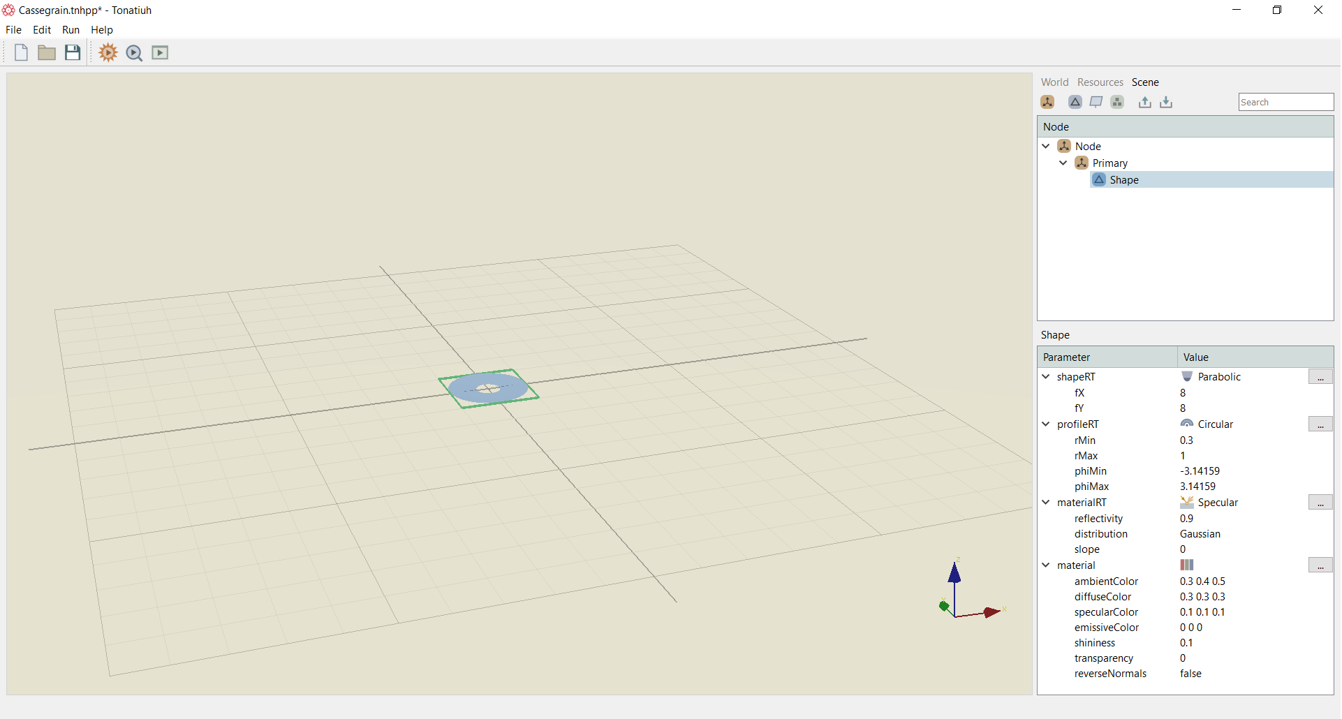
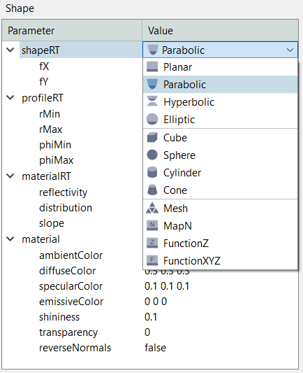
For the shapeRT parameter, press on the corresponding Value and a drop down menu will appear. From there choose Parabolic shape and for the focal length fx and fy set 8 as shown below.

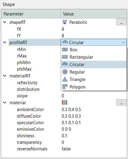
For the profileRT parameter chose Circular from the drop-down menu as shown below. For the rmin and rmax set 0.3 and 1 respectively.

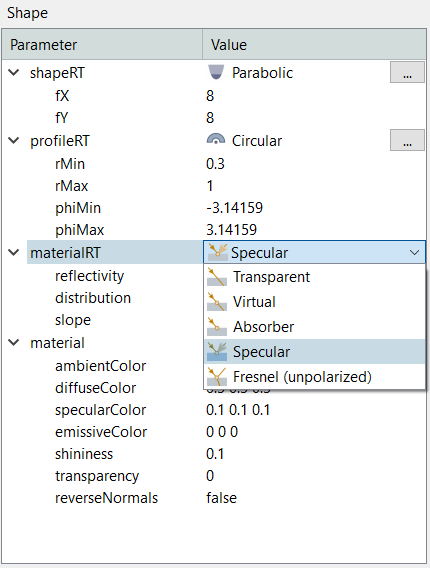
For the materialRT parameter set it as specular from the drop-down menu and set the reflectivity to 0.9 with Gaussian distribution and 0 slope.

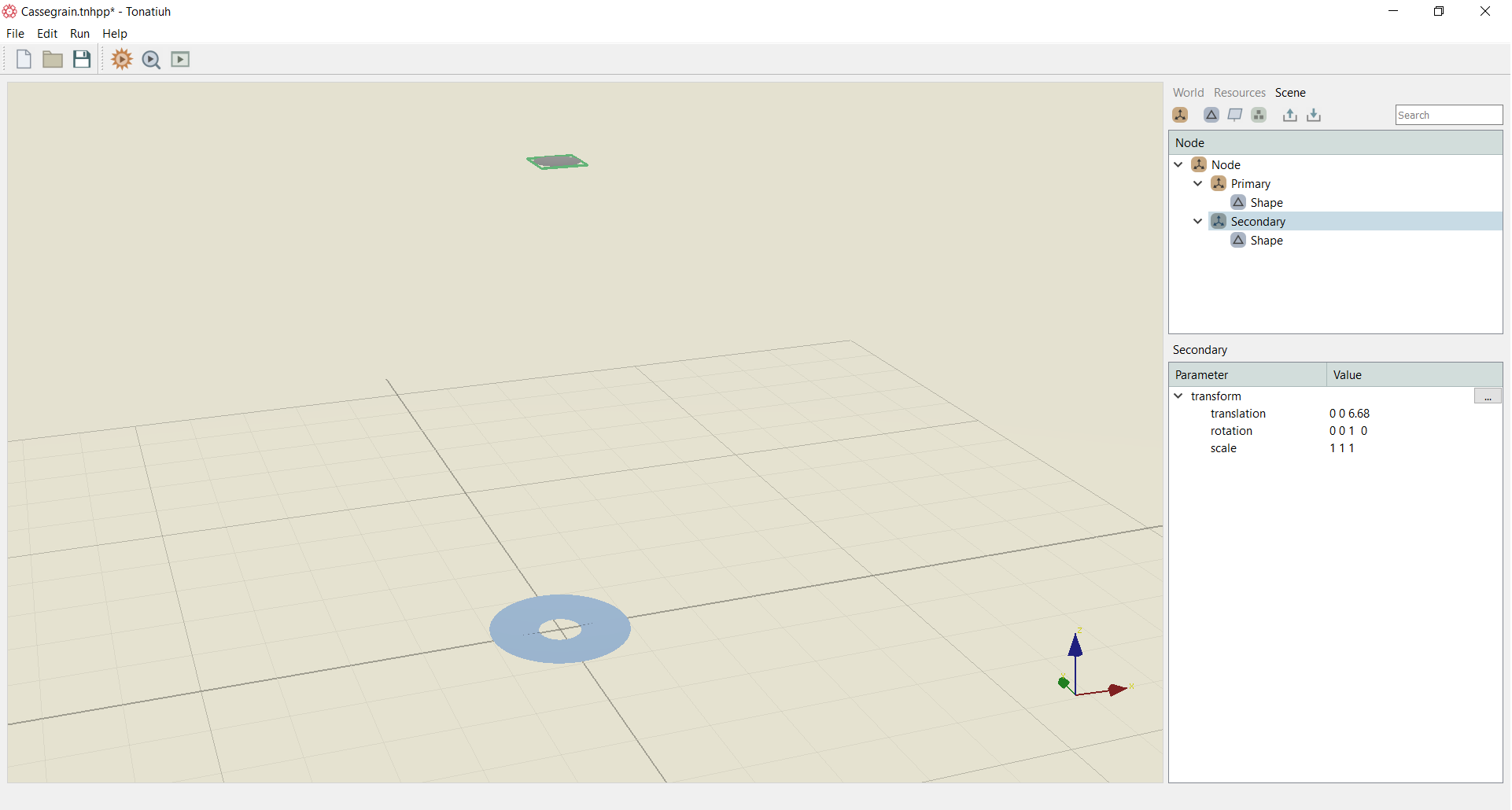
The primary mirror is set-up. For creating the secondary mirror, insert another Node and on the Node insert a new Shape as shown below. Now we need the secondary mirror to be translated by 6.68m above the primary mirror, thus set the translation to: translation 0 0 6.68 as shown below.

For the shape properties of the mirror, set a Hyperbolic shape with a Circular profile as shown below. Set also Specular for the material and set the reflectivity to 0.9 with Gaussian distribution and 0 slope as shown in Figure 8.

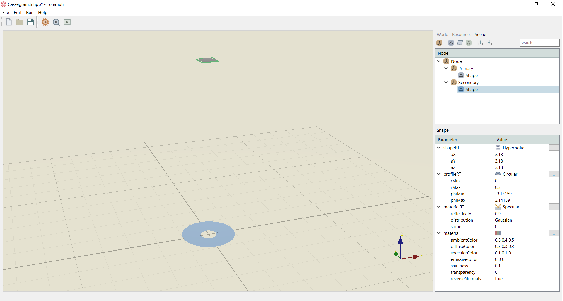
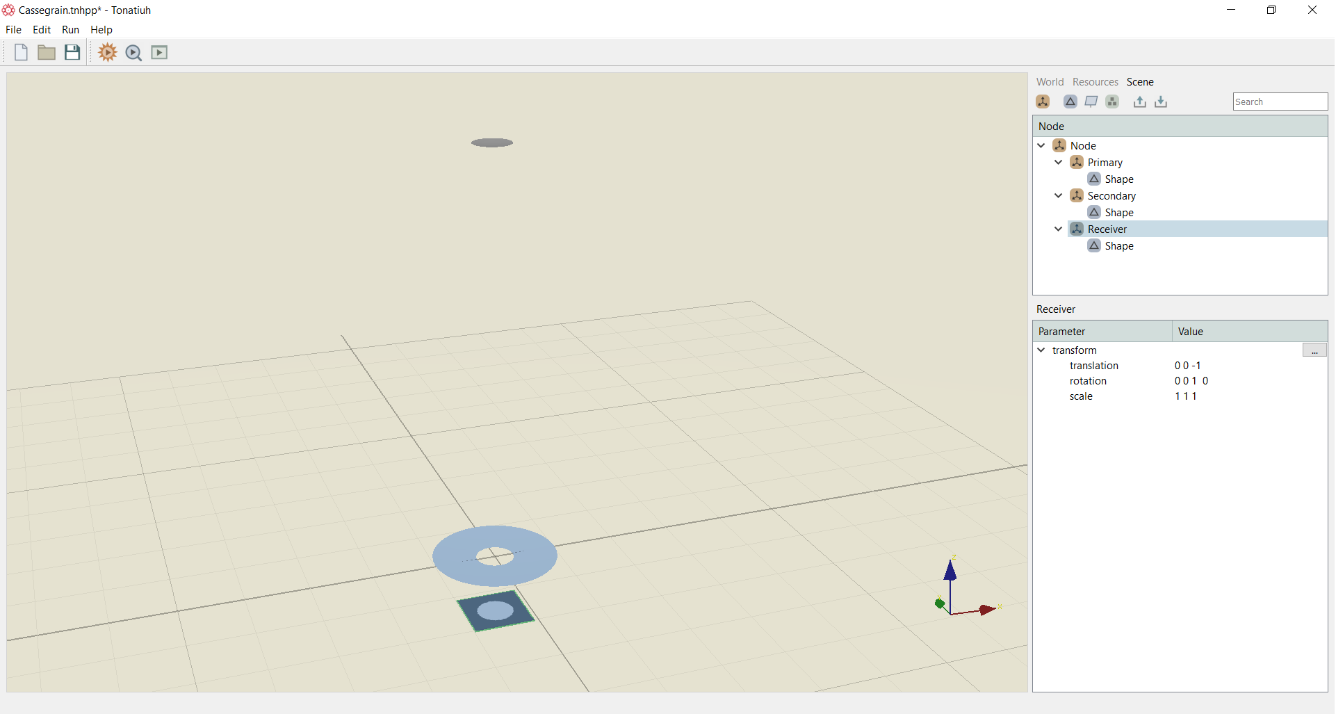
Finally, for the receiver, insert another Node and attach a new Shape on it. Translate the receiver 1m below the primary mirror by setting the translation to 0 0 -1 as shown below.

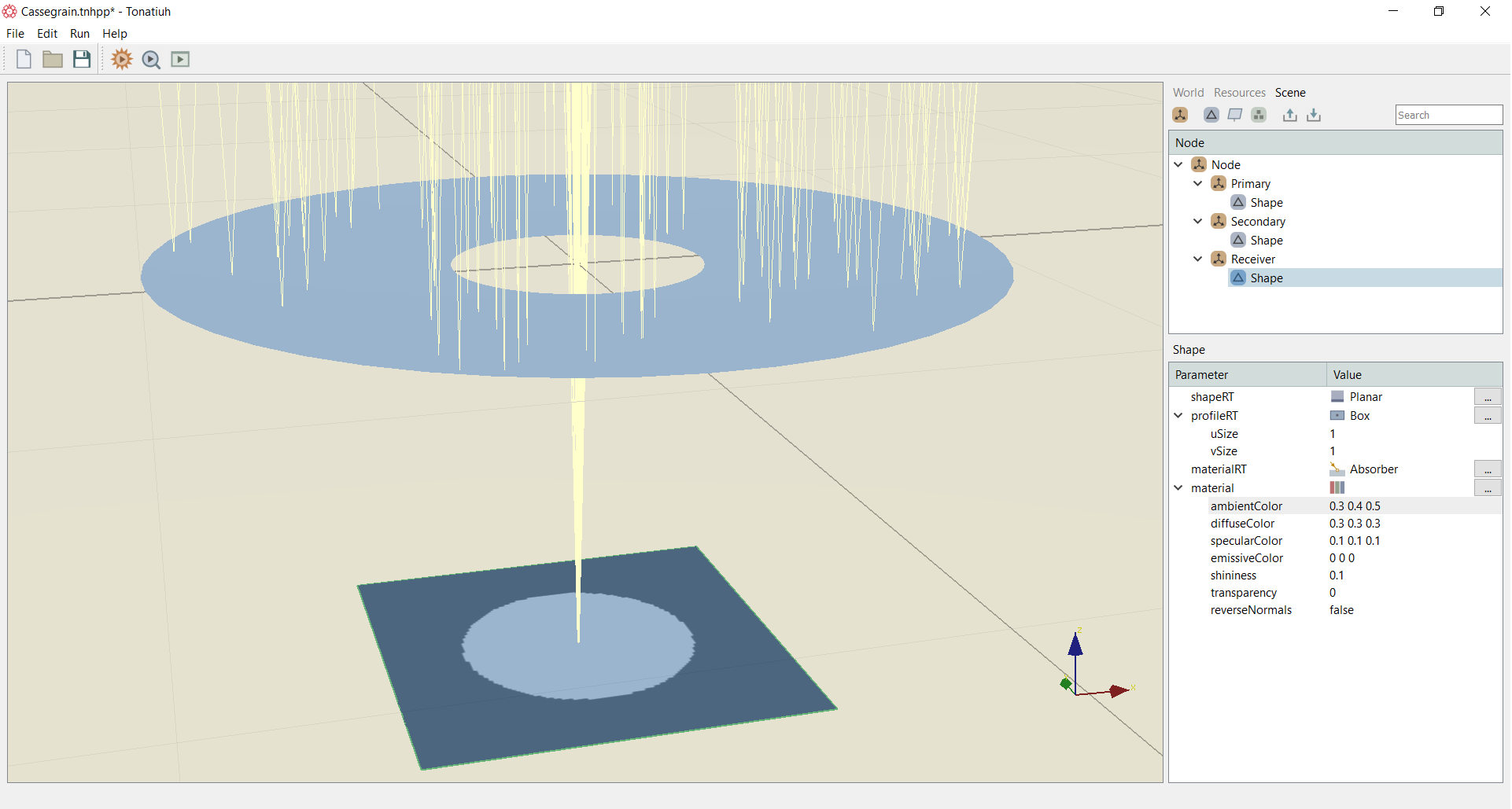
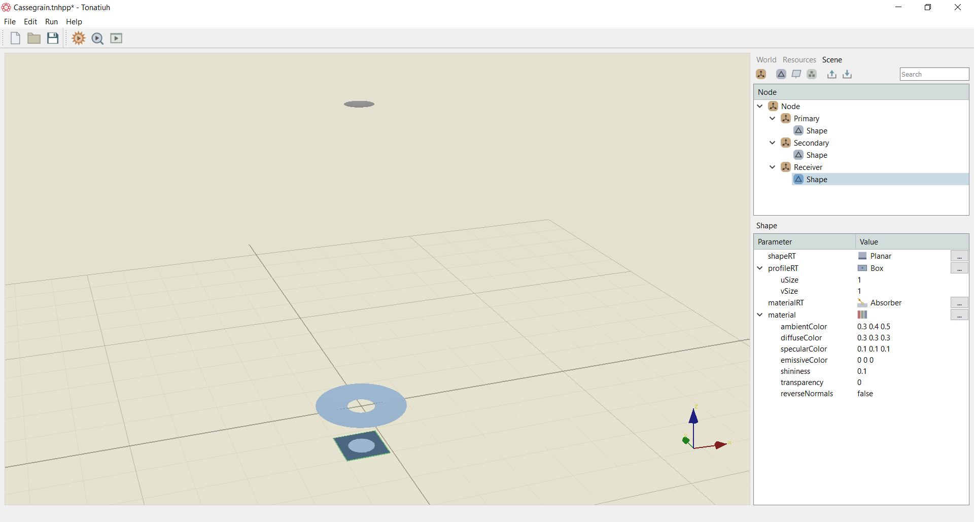
For the receiver's properties, use a Planar shape with a Box profile of size uSize 1 and vSize 1. Set the receiver as an Absorber as shown below.

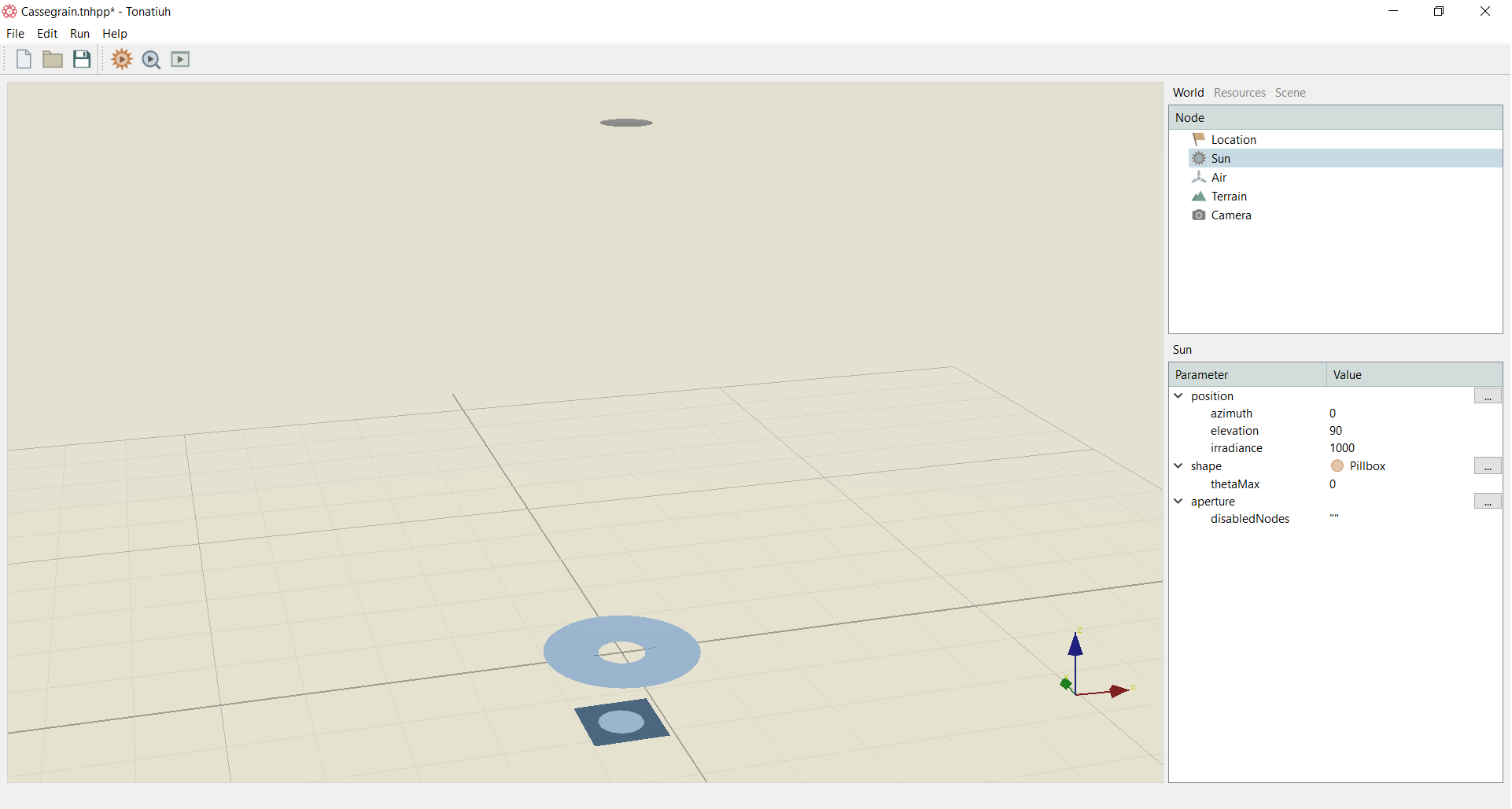
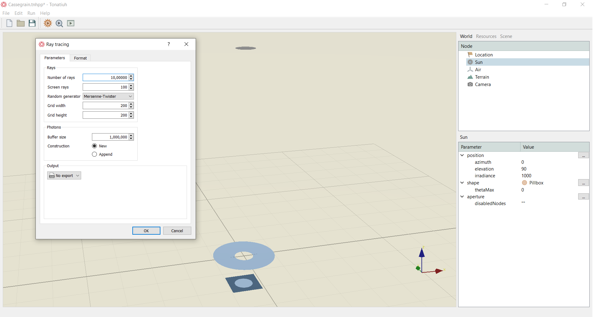
Now within the Graphics window you must have 3 components, the primary and secondary mirrors along with the absorber. Navigate to the World tab and set-up the sun parameters as shown below. Use Pillbox as the sun shape with thetaMax as 0, set azimuth to 0 and elevation to 90 with irradiance of 1000. For the location, terrain and air keep the default parameters.

Run the simulation by pressing the Run simulation button as shown below

You can see that the rays coming from the sun are reflect from the primary mirror towards the secondary mirror, and from there, the rays are reflected back down and are highly concentrated on the receiver.