11436160
Created by Ahmed Raza Hasan, last modified on May 04, 2017
R is a programming language optimized for working with data and performing statistical analyses.
Getting started in R via Jupyter Notebook is quite straightforward - simply create a new notebook using the drop down menu on the top right corner of the Jupyter interface, and select 'R'.
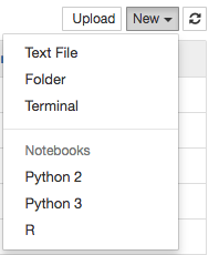
(Disclaimer: This wiki article is geared more towards intermediate R users who are looking to use the language more efficiently, and will not be covering the basics of how to program in it.)
A very common first step in R is to load more than one text file into the environment as a data frame object. The general way to go at it seems to be this:
df1 <- read.csv('file1.csv', header = TRUE)
df2 <- read.csv('file2.csv', header = TRUE)
df3 <- read.csv('file3.csv', header = TRUE)
And so on. While this process could be sped up with some copy pasting, it's still somewhat tedious and time-consuming.
Instead, we can use a loop and the assign() function to speed this up:
for (df in list.files()){
assign(df, read.csv(df, header = TRUE))
}
This will create data frames in your R environment out of everything in
your directory, which will automatically be named after their source
files. You can then take a peek at what's been loaded using the ls()
command.
If you'd rather only a subset of the files in your directory are loaded in as data frames, you can use wildcards in order to said desired files in. Perhaps the most common one is the asterisk (*), which matches anything of any length. For instance, if all my file names were of the format 'chromosome_', I could use this instead:
for (df in list.files(pattern = 'chromosome_*')){
assign(df, read.csv(df, header = TRUE))
}
If wildcards don't suffice, listing names out manually is also possible:
for (filename in c('a_file', 'anothercoolfile'){
assign(filename, read.csv(filename, header = TRUE))
}
One potential problem with this method is that the imported data frame
names often include the source file's extension. This is purely a
cosmetic issue, but it can be circumvented by using the paste()
function should it bug you. (It definitely bugs me.)
Let's imagine we have 17 files named chromosome1.csv through
chromosome17.csv. We could avoid having 'csv' stuck on the end of our
df names like so:
for (i in c(1:17)){
   dfname = paste('chromosome', i, sep='')
   assign(dfname, read.csv(paste(dfname, '.csv', sep=''),
                         header = TRUE))
}
This will create dfs that are just named 'chromosome1' through 'chromosome17' without the '.csv' tacked at the end.
So let's say we used the loop from above to import 17 different data frames into our R environment. Although the loop did help speed that part of the analysis up, now you have to run the same analysis over 17 data frames at once!
While one way to parallelize this is certainly to write an executable R
script that imports each file and performs any given analyses, sometimes
we just want to do some exploratory work with all our data frames in a
notebook. This process can be made significantly less painful by putting
our data frames in a list and making good use of lapply() ('list
apply').
lapply's syntax is pretty simple:
lapply(list, function)
And if our dfs are named 'chromosome1' through 'chromosome17', we can
pull them into a list pretty quickly using lapply() to begin with.
dflist <- lapply(ls(pattern = 'chromosome*'), get)
lapply works by applying an input function to every member of the
input list on an individual basis, and then returns to modified list
back to you. In this case, we're listing all the dfs in our environment
with ls(pattern = 'chromosome*') and then using the get function to
throw them all into a list.
Do be careful about the names of the dfs though - adding them to a list
can make them disappear for some godforsaken reason. This is quickly
remedied with the names function:
names(dflist) <- ls(pattern = 'chromosome*')
assuming your ls command is the same one you used to create the list
in the first place, since R will read them in the same order that way.
We can now define custom functions and run them in lapply:
thingdoer <- function(df){
    df <- do.a.thing(df)
    df <- df[which(df$col1 == df$col2),] # yes I know there's a dplyr way of doing this
    return(df)
}

dflist <- lapply(dflist, thingdoer)
Or even write quick and dirty functions in the body of lapply itself:
dflist <- lapply(dflist, function(df) df[which(df$col1 == df$col2,)])
One thing to be mindful of when working with lists of dfs is indexing. In order to access the underlying data frame in one of the list objects, make sure to index with two pairs of square brackets instead of one. For instance:
class(dflist[1])
 # returns 'list'
class(dflist[[1]])
 # returns 'data.frame'
Of the many wonderful things Hadley Wickham has blessed us with, the R pipe is one of the most consistently useful across the board.
It looks like this:
%>%
and what it basically means is 'take whatever is to the left of the pipe, and use it as input for whatever function is to the right of the pipe'.
So instead of typing:
answer <- foo(input)
answer <- bar(answer)
answer <- boo(answer)
answer <- far(answer)
or
answer <- far(boo(bar(foo(input))))
The pipe allows us to simply go:
answer <- foo(input) %>%
    bar() %>%
    boo() %>%
    far()
Notice how for each function after a pipe, we haven't explicitly typed out arguments. This is because the pipe will take whatever's on its left hand side and use it as input to said function, as mentioned earlier. Neat, huh?
If our function does have other arguments, those can be written in as normal:
hotspots <- chr12 %>%
    filter(mean > 0.1)
In this above example, filter is actually reading in
filter(chr12, mean > 0.1) as input.
By using the pipe, you can chain several operations onto a data frame together. This makes for more readable code and also saves time in actually writing up analyses.
The pipe integrates really well with the 'tidyverse', a suite of packages designed for efficiently working with data frames.
The signature tidyverse packages for df operations are called tidyr
and dplyr. Both contain a whole host of useful functions for reshaping
data, altering it, and more.
For this example, let's imagine we have a df of pairwise comparisons between genomic sites. We want to have R calculate the distance between each pair of sites, append that to a new column in the data frame, and also to filter out distances below 100 bp.
library(tidyr)
library(dplyr)

outdf <- df %>%
    distinct() %>%
    mutate(distance = position2 - position1) %>%
    filter(distance > 100)
This code will
1. Remove all duplicate rows from df (via distinct);
2. Create a new column called 'distance', whose values are calculated by
subtracting the value at position 2 by that of position 1, and append
that column to the df (via mutate);
3. Remove all rows whose distance value is below 100 (via filter).
4. Save the final product all the way back to a new df called outdf.
And it's actually pretty readable at the end of the day!
What I have here is barely the tip of the iceberg as far as both
packages' respective functions go. A handy visual reference for all the
cool stuff tidyr and dplyr are capable of can be found here. (Believe me when I say I
have literally never closed that tab.)
If you decide to make full-fledged R scripts to run on files in the terminal (highly recommended), making them executable is not difficult at all. Simply add
#!/usr/bin/env Rscript
at the top of the file, and you can then run it in bash with
Rscript [script].R
But what if we want to make our script take in arguments? Doing so is also easy enough. Add the following code to a script:
args <- commandArgs(trailingOnly = TRUE)
This will save all positional arguments given in bash to a list called 'args'.
So if the entirety of my script is just
#!/usr/bin/env Rscript
# this script is called test.R

args <- commandArgs(trailingOnly = TRUE)

print(args)
Then executing it in bash with some nonsense args returns this:
Rscript test.R hello hey 'how goes'
 # [1] "hello"    "hey"      "how goes"
Using commandArgs, you can therefore write (for instance) scripts that
will take in a text file, import it as a data frame, perform analyses on
it, and save a nice graph somewhere; and then proceed to run that over a
file in a directory somewhere with just something like:
Rscript makegraphs.R chromosome_1.csv
Or better yet, in parallel over files for the whole genome:
parallel -j 17 -i sh -c "Rscript makegraphs.R chromosome_{}.csv" -- {1..17}
Of course, it's also handy to have sanity checks in place when using
scripts. A useful way to have your script throw up an error if it
doesn't get the arguments it needs is by using the stop command.
Let's say this script needs 2 args. We can make sure that that's the case with:
if (length(args) != 2) {
  stop("Missing an arg", call. = FALSE)
}
If that stop function is executed, the whole script will immediately
break, potentially saving you lots of head scratching and frustration
down the line.
I'll be adding more stuff here as time allows! Feel free to update with your own nifty R tricks.
 Screen
Shot 2017-05-04 at 12.16.13 PM.png
(image/png)
Screen
Shot 2017-05-04 at 12.16.13 PM.png
(image/png)
Document generated by Confluence on May 22, 2024 11:44