Technical Specification Public Transit Supply
[1] Robinson et al (2013) “Modelling Demand in Public Transport in DynaMIT 2.0 and SimMobility: Technical Specifications” Tech_Specs_Public_Transport_Demand_DynaMIT_SimMobility_20130930.docx
[2] Robinson et al (2013) PUBLIC TRANSPORT DATA MODEL – TO BE FINALISED
[3] Oded Cats (2011) “Dynamic Modelling of Transit Operations and Passenger Decisions”. PhD thesis of Oded Cats, Department of Transport Science, KTH Royal Institute of Technology
[4] Burghout W. (2004). “Hybrid microscopic-mesoscopic traffic simulation”. Doctoral Dissertation, Royal Institute of Technology, Stockholm, Sweden.
[5] "DYNAMIT - Dynamic Network Assignment for the Management of Information to Travelers", (1998) Sridhar Rajagopal. Sridhar DynaMIT
[6] “Development of a Deployable Real-Time Dynamic Traffic Assignment System: DynaMIT Real Time programmer’s guide”. (2002)
[7] Steve Robinson (2013) “Desired Metrics for modelling Public Transport in DynaMIT and SimMobility”, DynaMIT design documentation
[8] Steve Robinson (2013) "Measuring Bus Stop Dwell Time and Time Lost Serving Stop Using London Buses iBus AVL Data", Accepted for publication in Transportation Research Record
[9] “Requirements for DynaMIT 2.0”, Requirements_DynaMIT_20130731.xlsx
[10] Cats (2008) "Mesoscopic Simulation for Transit Operations", MSc thesis Israel Institute of Technology
[11] Basak et al (2013) “SimMobility Integrated Simulation Platform: Public Transit in Micro & Meso level – 20th November 2013” Public Transit Micr Meso_20131120.docx
SimMobility includes the modelling of public transport. Several documents are being written to describe how this is achieved. For example there is a technical specification detailing how public transport demand will be modelled [9]. INCLUDE LINK TO OTHER SECTION
This technical specification focuses on how the movement of buses is modeled. This includes movement between bus stops, behaviour at bus stops, and modelling the dwell time at the stop.
This section provides a short literature review of modelling the movement of buses in a simulator. The first section discusses how bus travel time can be dis-aggregated into various parts. The second section reviews how public transport is simulated in various software. The third part provides a summary of how vehicles currently move within SimMobility. The last section gives a use case of the key processes in a block of vehicle journeys.
There are several papers with good literature reviews on dwell time. Rather than repeating the text here, the user is recommended to read the literature review in references [3] and [8]. Parts of the literature review of reference [3] are discussed in section 3.3.2 in the section on BusMezzo.
Typically the literature disaggregates travel time into two component parts:
- Drive Time: time the the vehicle is spent moving between stops
- Dwell Time: Time that the vehicle is spent stopped at the bus stop
A more comprehensive disaggregation of travel time has been suggested in reference [8]:
- Drive Time: Time spent moving between the stops assuming that no stops were present
- Deceleration Time: Time lost decelerating in order to serve the stop.
- Stationary time: This is the total time that the bus is spent stationary at the stop
- Door open time: This is the total time that the doors are open at the bus stop – i.e. when passengers are boarding and alighting
- Acceleration Time: This is the total time that the bus lost accelerating back to the drive time speed.
It should be noted that it is possible for the bus to the serve the same stop more than once. This commonly happens at very busy stops where there is a queue to access the front of the bus stop. In this scenario the driver may open the door once to allow passengers to alight the bus and some passengers to board. The driver will then drive forward slowly until the front of the bus stop is reached. The doors will then be opened again and more passengers allowed to board. Even if a bus stop is not crowded the driver may open the doors a second time to allow a new passenger who has just arrived at the stop the ability to board the bus. This suggests that the total stationary time and door open time is given, or separate times for each door opening. Additionally the following component of time is suggested:
- Creep time: This is the time spent by the bus moving from the first door opening to the last door opening at the stop.
This section describes how public transport has been modelled in existing software simulations. It firstly describes the different types of simulators. It then reviews a list of the most well know public transport simulators including BusMezzo, FastTrIPS, and Vissim.
There are three types of models commonly used in simulators which are briefly described here:
-
Microscopic: Model each individual entity explicitly in the simulation. The movement of each entity is determined solely from information available to the individual entity. In the context of modelling traffic, each vehicle will be modelled explicitly. The movement of each vehicle will be based on decisions made by the driver to accelerate, decelerate, or change lanes using a series of lane changing and gap acceptance models. These models have the ability to have good accuracy, but with high computation costs.
-
Macroscopic: Entities are aggregated together and not modelled individually. In the context of modelling traffic, demand will be modelled at the level of each OD, and estimates of the travel time through each link will be modelled using equations relating speed to the average density of traffic on the road. These models tend to be less accurate than microscopic models but are often orders of magnitude quicker to run.
-
Mesoscopic: Entities are implemented using both aggregated and disaggregated models. In the context of modelling traffic, demand will be modelled at a disaggregate level (i.e. individual passengers are modelled). However calculations on the travel time on a link will be undertaken at the aggregate level. The reasons for modelling at different levels of detail are:
-
Computational performance: macroscopic models are often orders of magnitude quicker than microscopic models
-
Accuracy: Microscopic models tend to provide more accurate simulations than macroscopic models
-
Data availability: Macroscopic models tend to require less detailed information about the network.
Therefore the decision on what level to model is primarily a trade off between accuracy and computational speed. There is therefore a requirement to know how accurate the results need to be when making a choice of how to model the various entities. Software that simulates public transport has been implemented using microscopic, mesoscopic, and macroscopic models. Some of these are described below.
BusMezzo is a dynamic transit operations and assignment model, that simulates and evaluates the operation of Public Transport [3]. It is integrated with the Mezzo road simulator. It is probably the most comprehensive implementation of a public transport simulator to date. BusMezzo and Mezzo differ from DynaMIT in that they are event based simulators. BusMezzo models bus travel time as being the summation of riding time between stops and dwell time. It should be noted that the definition of dwell time includes the component of travel time spent decelerating and accelerating to the stop.
3.3.2.1 Riding time between stops
The riding time of the bus is modelled in the same way as the standard Mezzo, with events generated to model the bus entering and exiting links, as well as entering stops. This is the key difference with DynaMIT which uses a time-based approach.
In BusMezzo the speed on the link is determined using a speed-density relationship.
3.3.2.2 Dwell time
The dwell time models in BusMezzo are a feature which Mezzo does not have. Bus dwell time in BusMezzo is given by the folowing equation.

DTs,l,k,f = Dwell Time at stop s on line l for trip k and vehicle type f
lost_times,f = constant delay time for stop s and vehicle type f to take into account time lost accelerating and decelerating from the stop s
PSTs,l,k,f = Passenger service time
vs,l,k,f = error term
Lost time is given in more detail in the below equation.
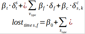
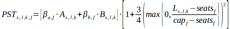
In this equation the first term corresponds to the fixed delay of visiting a stop. The second term corresponds to increased fixed delay caused by different stop types (e.g. bay stops have more delay usually than in-road stops). The third term corresponds to increased fixed delay caused by differing vehicle types (e.g. some buses have slower acceleration). The fourth term corresponds to additional delay caused by the bus having to queue at the stop. This was added so that the vehicle movement logic of Mezzo would not have to model this.The passenger service time (PST) gives the time taken for all the passengers to board and alight from the bus. BusMezzo allows the end user to choose from four such models. Two of these will be described below. The more basic of these gives the PST assumes the bus has two doors, one for entering and one for existing, and gives the PST as the maximum of the total alighting time and the total boarding time. It is given by equation below:

A more advanced equation of PST takes into account how crowded the bus is and is given by the below equation.
DynusT (Dynamic urban systems for transport) is a traffic simulator developed at the University of Arizona. It is an offshoot of the DynaSMART traffic simulator.
TO BE FINISHED
TO BE FINISHED
The objective of this work is to integrate Public Transport into SimMobility. It is therefore necessary to ensure that the solution on moving buses proposed is compatible with the existing supply simulator of SimMobility. This section provides a short review of this. A more complete review of the movement of a vehicle in a link is described in section 2.3 of reference [5] and section 11 of reference [6].
A list of the key principles in the movement of vehicles in SimMobility is given below:
Every vehicle is modeled explicitly in the network as a packet. The location of the vehicle is denoted by the segment ID and the distance traveled along the segment id
Each vehicle is moved along the network every “advance phase”. This value is configurable and currently set to 5 seconds.
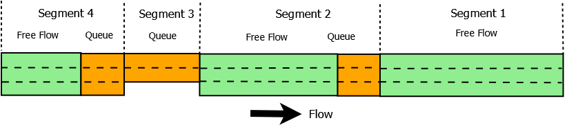
Each segment is dis-aggregated into a “moving” section with a “queuing section” at the end of the segment. The total travel time in the segment is given by the travel time through the “moving section” plus the travel time through the “queuing section”. This is illustrated in the following figure.
This section defines a common glossary that will be used throughout the technical specification documents. This is particularly necessary when modelling Public Transport as certain words can mean different things to different people – in particular the words “route” and “trip”.The glossary is in alphabetical order.
| Word | Description |
|---|---|
| Access Walk | This is the movement of a person from their origin point to the first stopping point in the trip |
| Block | Describes the sequence of vehicle journeys scheduled to be performed by the same PT vehicle on any given operational day |
| Direction | Determines which way of the line the vehicle journey is running in e.g. direction 1 = Bedok to NUS, direction 2 = NUS to Bedok |
| Duty | Reference to an arbitrary driver. On a given operational day a specific person (driver) will be allocated to a given duty. This is similar to the concept of a block number which references an arbitrary vehicle |
| Egress Walk | This is the movement of a person from their last stopping point in the trip to their final destination D |
| Line | A service which is known to passengers by a common number or name. For example the “33” is a line between NUS Kent Ridge and Bedok, operated by a bus |
| MRT | Mass Rapid Transit system. The name of Singapore’s urban rail network. It should be noted that since 2011 Singapore does not have an overground network |
| Operational Day | This describes a day used in a schedule. An operational day allows for the fact that vehicle journeys on a line can straddle two calendar days or even start after midnight. A 29 hour day is typically used with timings after midnight having a start hour more than 23. An Operational day runs from around 02:00 to 05:00 the next Calendar day – i.e. 02:00 to 29:00 |
| Path | Describes the sequence of access walk, rides, transfer walks, and egress walks that a passenger took on a trip |
| Pattern | Describes the exact sequence of stopping points that a PT vehicle takes on a given vehicle journey. Typically a line has two patterns, one in each direction. If a line has short working vehicle journeys then there will be more than one pattern for the line-direction |
| Ride | Describes a single movement on a single vehicle carried out as part of a Trip |
| Stand | A location where a PT vehicle will wait in between in-service vehicle journeys |
| Stopping Point | Describes a location where a passenger may board or alight a Public Transport vehicle. In practice this is either a bus stop or platform |
| Transfer Walk | Describes the movement of a passenger between different vehicles in a trip |
| Trip (PT Trip) | Describes the movement of a person between an origin point O, and a destination point D |
| Vehicle Journey | An instance of the service on a given line provided between a starting stopping point A and end stopping point B |
It is important to review the requirements for modelling the movement of public transport. This chapter reviews these requirements. This work also builds on earlier design work stated in references [7] and [9]. The first section reviews what output data is required from the SimMobility supply simulator when modelling the movement of public transport. The following sections then list other requirements. Section 4.5 provides a use case of modelling a block of trips. This use case provides a very good reference against which to validate the solution and to ensure that all functionality is being provided.
A summary of all the data outputs required from the supply AND demand simulator is given in table below. The output files for each entity must be common between the short term and mid term simulator. However some attributes will only be available in the Short Term simulator. These are indicated by a ‘*’. The “model used” attribute can be used to indicate if the data came from a short term or mid term simulator.
| NO | NAME | DESCRIPTION |
|---|---|---|
| 01 | PT vehicle stopping point observation | Every time a Public Transport vehicle departs from a stopping point a record with the following attributes must be provided: - Vehicle id - Vehicle Journey Id (including operational day,,line, etc) - Stop Point id - Sequence in vehicle journey - Scheduled Arrival time - Scheduled Departure time - Observed Arrival time - Observed Departure time - List of Passengers boarding - List of Passengers which failed to board - List of Passengers alighting - List of Passengers on board - Dwell time - Time lost arriving** - Time lost departing** - Model used NB. Terms marked by ‘**’ may be implemented at a later date |
| 02 | Public Transport Vehicle Location | Every x seconds each PT vehicle should output information about its location. The attributes of each vehicle location record are given below: - Vehicle id - Timestamp - Location of vehicle: Local (see requirement 11)* - Location of vehicle: WGS84 (see requirement 12)* - Location of vehicle: Linear Reference System (see,requirement 13) - Vehicle journey id - Heading in degrees* - Speed in kph - List of passengers on board - Model used |
| 03 | Stopping Point Status | The supply simulator must be able to output the following information at each stopping point at each advance phase: - Stop Point id - Timestamp - List of Passengers waiting at the stop - Model Used |
| 04 | Bus Arrival Prediction | A “Bus Arrival Prediction” provides a prediction of the arrival time of a bus at a bus stop. There is a single record for each combination of bus, journey id, and stopping point id. The attributes in each record are given below: - Vehicle id - Vehicle journey id - Stop Point id - Timestamp that prediction was made - Predicted Arrival Time - Model used |
| 05 | Stop Link Status | A “Stop Link” describes the section of road between two adjacent stopping points on a transit line. Every x seconds the status of each “Stop Link” will be provided in the “Stop Link Status” object. The attributes of this object are given below: - Start Stop Point - End Stop Point - Timestamp - Travel time - Model Used |
| 11 | PT Trip | A “PT Trip” describes a series of rides made by a passenger so that they can travel between a given origin and destination. For every PT trip completed the following attributes will be output in a record: - Passenger Id - Timestamp trip started - Timestamp trip ended - Origin location - Destination location - List of completed rides, access, egress and,transfer walks |
| 12 | Ride | For each completed Ride the following data will be output: Passenger Id PT Trip Id Timestamp boarding Timestamp alighting Stop Point boarding Stop Point alighting Vehicle Id Vehicle journey id Line Id |
| 13 | Walk: Access, Egress, Transfer | For each completed transfer walk the following data will be output: - Passenger Id - PT Trip Id - Type of walk: access, egress, or transfer - Timestamp departed start stop point - Timestamp arrived end stop point - Stop Point start: can be null for access walks - Stop Point end: can be null for egress walks - Location start: can be null for egress or transfer walks - Location end: can be null for access or transfer walks |
| 21 | Location in local format | The system must be able to provide the location of a vehicle in local coordinate system |
| 22 | Location in WGS84 format | The system must be able to provide the location of a vehicle in WGS84 format |
| 23 | Location of vehicle: Linear Reference System | The system must be able to provide the location of a vehicle using a linear referencing system. Typically this will include the following attributes: - Segment Id - Distance from start of segment |
| 31 | Format of data | All records stated above shall be stored as UTF-8 files. These files can be compressed as required |
| NO | NAME | DESCRIPTION |
|---|---|---|
| 201 | Common Design | The SimMobility mid-term software and DynaMIT should share as much code reasonably possible in the modelling of public transport |
| 202 | Calibration | The system should allow the position of buses in the system to be corrected using real time bus AVL information |
| 211 | Accurate | Most users of SimMobility and DynaMIT 2.0 will only require very accurate predictions on certain parts of the network. |
| 212 | Computationally quick | Given the scalability challenges that DynaMIT 2.0 will face, it is desirable to model each entity as computationally efficiently as possible. |
| 213 | Data availability | Data required to model bus stops to great detail, such as the bus stop type and length, may not be available. Therefore the solution should be robust to less than perfect data |
| NO | NAME | DESCRIPTION |
|---|---|---|
| 301 | Common Mode design | A common design for modelling MRT and buses should be used where possible. |
A list of bus specific requirements for the modelling of Public Transport is given in the below table
| NO | NAME | DESCRIPTION |
|---|---|---|
| 401 | Overtaking at stops | The system must allow for buses to overtake one another at bus stops |
| 402 | Queuing at stop even with space available | The system must take into account the reluctance of bus drivers to stop at a bus stop immediately ahead of a bus already stopped at the stop |
| 403 | Bus stop types | The system must be able to take into account the different type of bus stops typically encountered (on road, bus bay, bus station) |
| 404 | Bus types | The system must support different bus types that will have varying:,Length,Capacity,Height |
As a validation stage in eliciting requirements it is useful to produce a flow diagram indicating the key processes in the movement of a bus in a block of vehicle journeys (refer to section 3.5). This flow diagram should indicate all possible processes that might occur and should therefore be incorporated into the design. Such a diagram was produced and is shown in the following figure. There are three main “actors”:
- Controller: This is a manager who is in overall charge of the operation of the line
- Vehicle: This is the actual PT vehicle
- Driver: This is the person who operates the PT vehicle
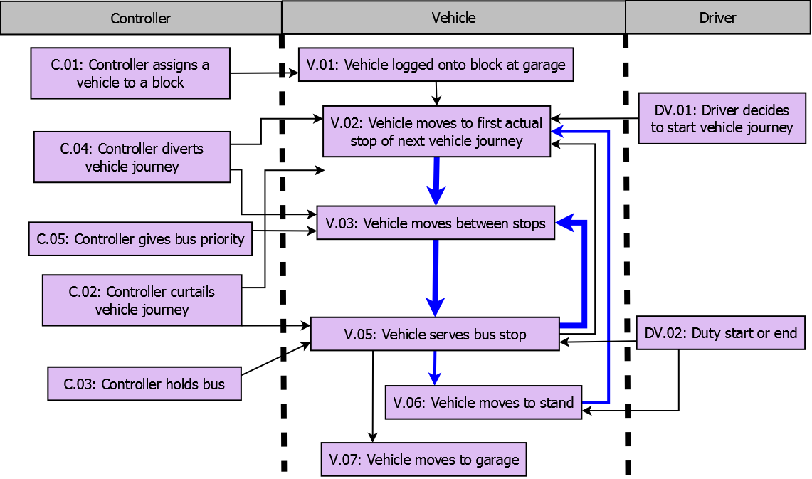
Each process is described briefly in the table below. The primary flow refers to processes which will definitely occur. The “alternative flows” refers to processes which may or may not happen.
| Name | Description |
|---|---|
| Primary Flow | |
| C.01: Controller assigns a vehicle to a block | The controller begins the use case by assigning a PT vehicle in the garage to a block number in the schedule. It should be noted that the block will consist of a sequence of in-service journeys (where passengers are allowed) and out-of-service journey (where passengers are not allowed on the bus) |
| V.01: Vehicle logged onto block at garage | The PT vehicle will then be logged into the block so that the PT vehicle now has a sequence of scheduled vehicle journeys to perform during the day |
| DV.01: Driver decides to start vehicle journey | The first vehicle journey should begin at the scheduled start time. However this is dependent on the driver ensuring this happens. The driver might start early or late depending on his mood and other necessities. |
| V.02: Vehicle moves to first actual stop of next vehicle journey | The vehicle will move to the first stopping point of the next vehicle journey. |
| V.03: Vehicle moves between stops | The vehicle then moves from one stop to the next along the road or track. |
| V.05 Vehicle serves bus stop | As the vehicle passes a stop it will serve it. If passengers wish to alight or board the bus then the bus will stop and allow them to do so. Otherwise the bus will continue. MRT trains will stop at all scheduled stopping points. |
| V.06: Vehicle moves to stand | Once the in-service vehicle journey has been completed, the vehicle will then move to the stand |
| V.07: vehicle drives to garage | Once all in-service vehicle journeys have been completed the vehicle will return to the garage. |
| Alternative Flows | |
| DV.02: Duty start or end | At certain points within a vehicle block the driver will be changed.,This typically occurs at stands but can occur at any point in the route. |
| C.02: Controller curtails a vehicle journey | If a vehicle journey is badly behind schedule or there is bunching on a line then the controller may decide to prematurely end a vehicle journey so that the service in the other direction will not be badly impacted. |
| C.03: Controller holds bus | The controller may choose to force a bus to remain stationary at a bus stop. This is either to ensure the bus does not leave the stop early. |
| C.04: Controller diverts vehicle journey | The controller can choose to divert the vehicle journey if there is an accident or other blockage on the scheduled path. |
| C.05: controller gives bus priority | The controller can give the vehicle priority at some locations in the network.,For example UTC systems can give buses priority at traffic lights. |
These processes act as a good set of requirements and reference model against which the proposed design can be checked against.
This section provides an overview of how it is proposed to model the movement of buses
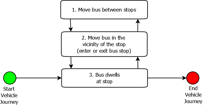
Elaborating on the use case described in section 4.5 it can be seen that there are three stages of movement that have to be considered which are illustrated by the following figure.
- Stage 1: Moving between bus stops
- Stage 2: Moving in the vicinity of the bus stop. This can be split into three parts:
- Entering the bus stop
- Leaving the bus stop and re-join the main traffic stream
- Interaction between bus stop and surrounding traffic stream (queue spillback) - Stage 3: Dwell time of the bus at the bus stop.
This section describes in detail stage 2 of above figure, i.e. the movement of buses in the vicinity of a stop. It describes the different types of bus stops, provides the attributes of a bus stop, and introduces the concept of a “virtual stop” to show how each type of stop should be modeled. It then describes how buses move into and out of the bus stops.
There are typically three major types of bus stops which need to be modeled. These are described below. For each bus stop type an indication of where queuing might occur for other traffic is indicated.
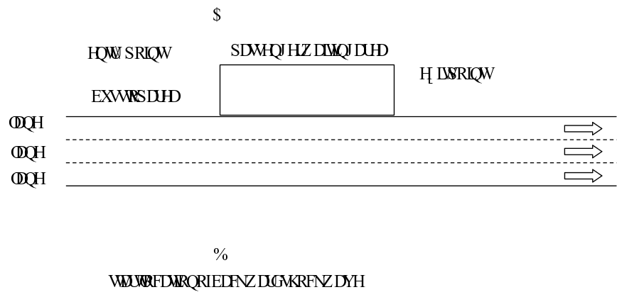
6.1.1 On-road bus stop
The first type of bus stop is an on-road bus stop and is illustrated in the following figure. Buses will stop on a normal traffic lane temporarily blocking that lane. The front of the bus stop is typically marked by a flag. Drivers are trained to open the front doors next to the flag when possible. The length of this bus stop is typically not well defined as it depends partly on the driver making a decision as to where the stop starts and ends.
The second type of bus stop is the bus-bay type and is illustrated in figure below. In these layouts there is typically a small lane added by the side of the road which the buses move into before opening their doors to allow passengers to alight and board. The length of these bus stops is clearly defined by the length of the bay.
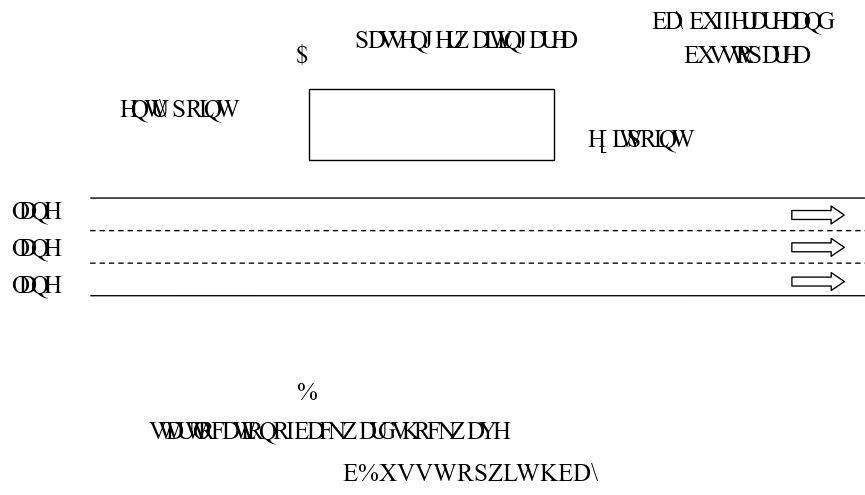
Queuing will occur on these bus stops when the bus bay is full and a bus has to wait at the rear of the bus stop to enter the bus stop. Therefore the line AB is defined at the rear of the bus bay.
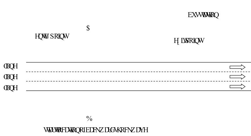
The final type of bus stop is the bus station and is illustrated in the figure below. Bus stations are located away from the main road links. Typically a node will have been defined for the entrance and exit of a bus station to the main road network. The capacity of a bus station, can for all practical purposes, be deemed as unlimited, so queuing is not expected at AB.
The number of buses that can be served by a bus stop at any one time is defined as the storage capacity of the bus stop. The capacity of a bus stop is dependent on the length of the bus stop. Typically the planned capacity of the bus stop is given by the length of the bus stop divided by the average length of a bus.
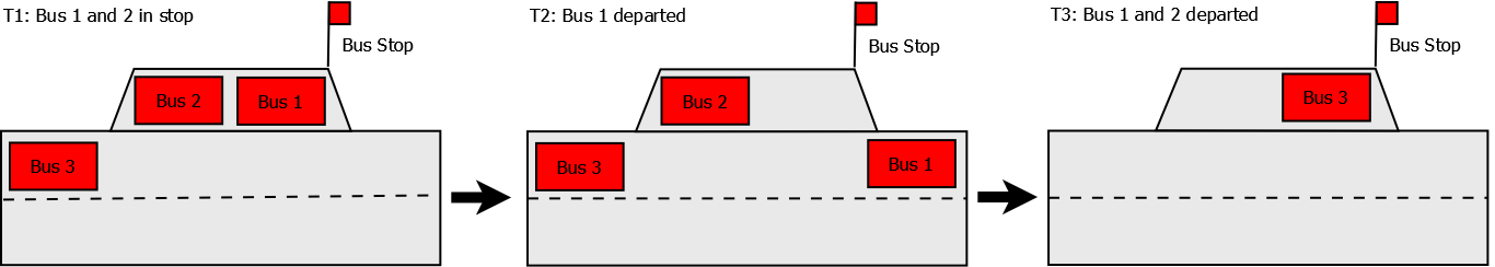
However, in reality the effective capacity is typically less than this planned capacity. This is because buses will not optimally use the length of the bus stop. As an example, Figure 7 shows bus #3 wanting to serve a bus stop. However in the first time step T1 there are already two buses at the stop so it cannot enter. In time step T2 bus #1 has departed. However buses entering a bus stop tend to be reluctant to overtake a bus already at the stop as they will not be able to align the bus close to the pavement. The driver is therefore likely to wait until bus #2 has departed. In time step T3, bus #3 then chooses to stop at the front of the bay.
A small study could be undertaken to observe and validate such rules.
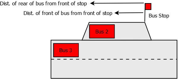
For each bus in the stop it should be possible to calculate the following:
- Distance between front of bus and front of virtual stop
- Distance between rear of bus and front of virtual stop
- Time that this bus will depart the stop, in seconds
These are illustrated in the following figure.
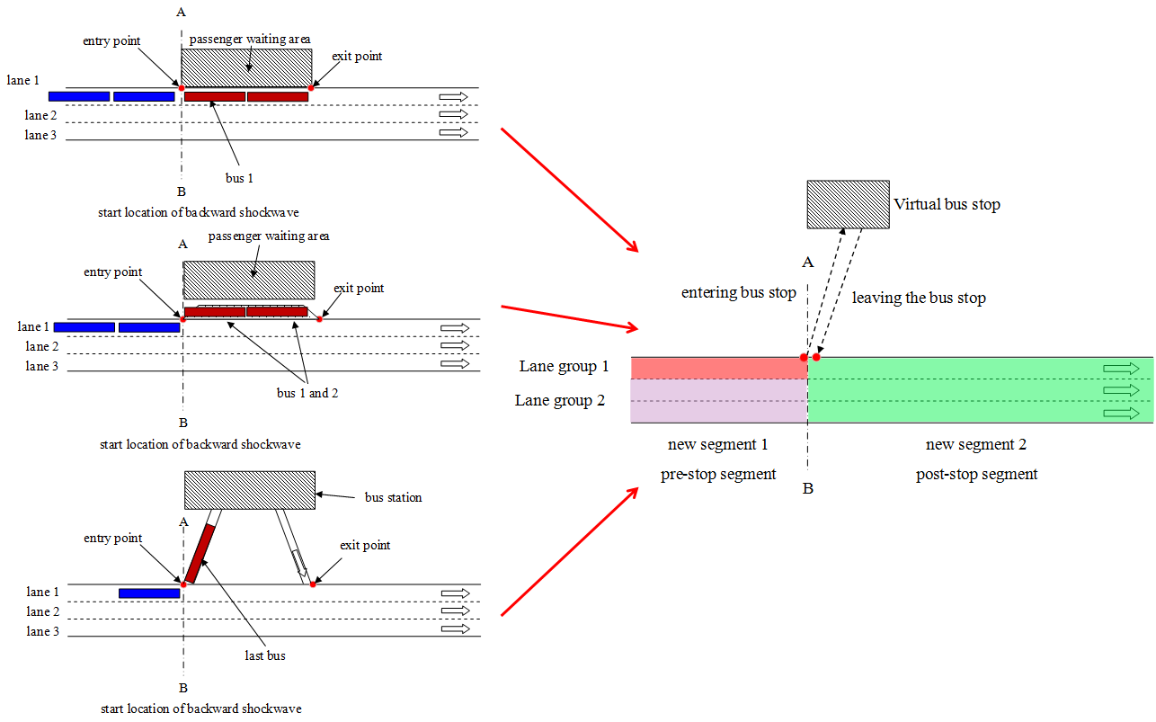
Three important design concepts regarding modelling bus stops in existing DynaMIT network structure are proposed:
- Concept 1: By splitting the original road segment (with single bus stop) into two new segments from the location of entry point (shown by AB), DynaMIT can fully capture the potential impact of queue spillback from the bus stop;
- Concept 2: The operational characteristics of all three types of bus stops can be modelled uniformly with a single logical unit if designed properly. (The logical unit is called a virtual bus stop)
- Concept 3: Buses can only enter a virtual bus stop if there is spare capacity in the virtual stop.
This section summarises how bus stops will be modelled in SimMobility. There are two key stages; network re-segmentation and creation of a “virtual stop”.
The first approach to modelling bus stops in SimMobility is to split the existing segment where a bus stop is located. The split will occur at the location AB given in the above figures. This process is illustrated by the figure below.
In this diagram it can be seen that the existing segment is split into two at the location where queuing may form due to the presence of the bus stop. This is indicated by the lines AB in the figure. A “virtual bus” stop is defined at the intersection between the two segments – i.e. at AB.
The second stage is to create a “virtual stop”. The characteristics of a virtual stop can be split into static and dynamic fields and are given below:
Static Attributes:
- Type: The type of bus stop: on-road, bus-bay, bus station
- Length: length of the stop in metres. It is used to indicate the storage capacity of the stop
- Planned bypassing capacity: This is a binary flag to indicate if a vehicle can exit from the outer most lane of the upstream segment into the downstream segment. For bus stations and bus bays this is always 1, indicating that a parked bus in the stop does NOT block other traffic. However for on-road bus stops this is zero indicating that when a bus is in the virtual stop then other traffic in the outer lane of the upstream segment will be blocked by the bus.
Dynamic Attributes: - Receiving capacity RB(t): Indicates whether there is room in the virtual bus for more buses at time t.
- load of the bus stop L(t): Current load of the bus stop
- Bypassing capacity, P(t): Indicates whether at the current time vehicles in the outer lane of the upstream segment can move into the downstream segment.
- Discharge rate, D(t): This is discharge rate from the virtual bus stop back into the main traffic stream. It should be noted that when the bus is in the virtual stop it is removed from the road segment.
6.5 Moving buses into a bus stop
This section describes how buses move from the upstream segment into the virtual stop. The process is illustrated by figure below where:
- S1(t): Output capacity of new segment 1, lane group 1
- R2(t): Receiving capacity of new segment 2:
- RB(t): Receiving capacity of virtual bus stop:
- P(t): Allowed bypassing capacity from new segment 1 to 2: either 0 or 1
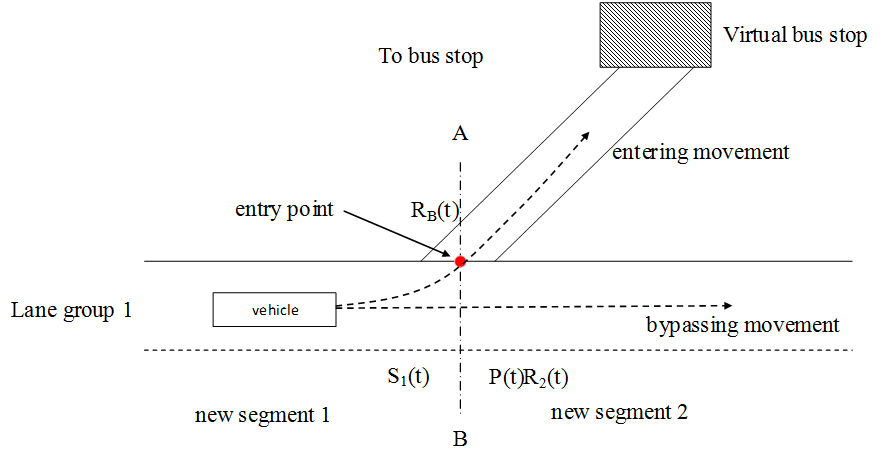
The condition for the bus to enter the virtual stop is:
- S1(t) > 0 AND RB(t) > 0
The condition for a vehicle to bypass the stop is: - S1(t) > 0 AND P(t)·RB(t) > 0
The business rules stated in section 6.2 can be used to determine the receiving capacity of the virtual bus stop, RB(t).
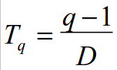
This section describes how buses move from the virtual stop back into the downstream segment. The process is illustrated by the following figure.
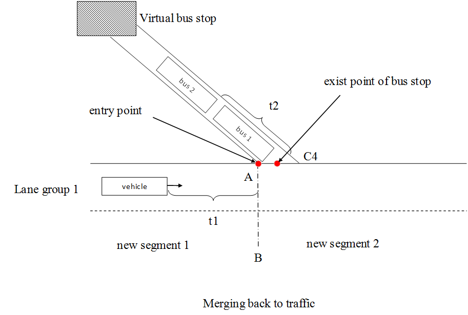
The time taken for the position ‘q’ bus waiting to return from the virtual bus stop to segment 2, is given by equation below:
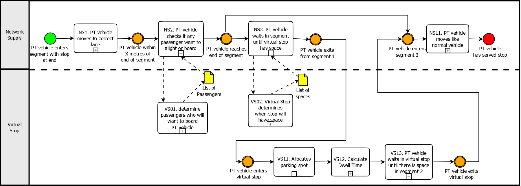
A Business Process Modelling Notation diagram showing the process of a bus in the vicinity of a bus stop is given in the figure. Each process is described in the table. It should be noted that there are two key actors:
- Network Supply: This actor represents the existing SimMobility code which moves vehicles through the network. The network supply manages the bus between bus stops and manages the entry of the bus into the virtual stop.
- Virtual Stop: This actor represents the new virtual stop entity. It manages the dwell time of the bus and also the return of the bus back into the network.
| Process name | Description |
|---|---|
| NS1. PT vehicle moves to correct lane | The use case begins when the PT vehicle enters a segment which has a bus stop at the end. If the bus is scheduled to serve the bus stop then it will choose the outer most lane – i.e. the lane with the bus stop. If a bus is NOT scheduled to serve a bus stop at the end of the segment then the bus is free to choose any lane like other vehicles. |
| NS2. PT vehicle checks if any passenger wants | When the vehicle is within X meters of the end of the segment a check is made whether any passengers on board the bus want to stop at this stop. A call is made to VS01 to see whether there are any passengers at the stop who would like to board the bus. If no passengers want to alight or board the bus then the bus will NOT serve the bus stop. In this case the bus will remain in the outer most lane until the end of the segment is reached and then move directly into segment 2. |
| VS01. Determine passengers who will want to board the vehicle | The Virtual Stop determines which of the passengers waiting at the stop will want to board the bus. |
| NS3. PT vehicle waits in segment until virtual stop has space | If,there are passengers that want to either alight or board the PT,vehicle, then the vehicle will wait at the end of segment 1 until,there is space to enter the stop. This is determined by making a,call to VS02. This process is described in more detail in,section 6.5. |
| VS02: Virtual stop determines when stop will have space | The virtual stop determines how long waiting buses must wait until there there will be space for a bus to enter the bus stop. It returns a list of expected waiting times for when spaces will be free. There will be one record for each bus currently parked in the virtual stop. If there are no buses in the stop then the returned list is empty and the supply simulator assumes a 0 second wait time. For each bus in the stop the following is returned as illustrated in Figure: Distance between front of bus and front of,virtual stop,Distance between rear of bus and front of virtual,stop,Time that this bus will depart the stop, in,seconds,NB. The concept of the parking place in the virtual stop was described in section 6.2. It should be noted that the supply simulator must have knowledge of the length of the stop |
| VS11 Allocates parking spot | Once there is space available in the virtual stop, the bus is allocated a parking spot. Refer to section 6.2. |
| VS12. Calculate Dwell Time | The dwell time of the bus at the stop is then calculated. Refer to section 7. |
| VS13. PT vehicle waits in virtual stop until there is space in segment 2 | After the dwell time has been completed the time that the bus has to wait to return to the main traffic stream is then calculated. This will depend on the bus stop type. The logic of this is given in section 6.6. Once this time has elapsed the PT vehicle enters segment 2. |
| NS11. PT vehicle moves like normal vehicle | Once the PT vehicle has returned to the main network, it continues to move towards the next scheduled bus stop. |
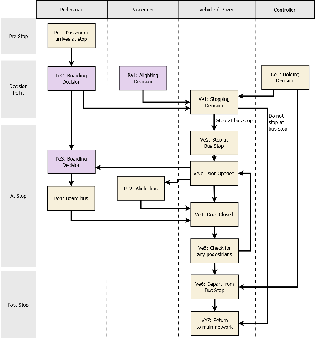
This section elaborates on the interaction between the supply and demand simulator at the bus stop. Travellers must make a decision to board a bus and a decision to alight a bus. This section indicates where these decisions are made. An overview of the processes that take place at the bus stop is given in figure below. This will be explained in more detail in the table. It shows how each of the important actors in the system behave. These actors are:
- Pedestrian: a person waiting at the bus stop who wants to board the bus
- Passenger: a person at the bus stop who wants to alight the bus
- Vehicle / Driver: the agent in charge of moving the vehicle
- ContollerController: The service controller who instructs the driver on headway and trip curtailments.
There are four key time periods: - Pre-Stop: This is the time before the bus reaches the decision point
- Decision point: This is the time the bus reaches a point in the road where the drive must make a decision on whether to halt the bus at the stop. This should be configurable for the stop with a default value of 20m when the bus is travelling at normal speed. This takes into account the distance required to break at a speed of 30kph. In congested traffic this point may be closer to the bus stop. NB. For simplification purposes the default offset distance could also be made 0m for ALL stops.
- At stop: this is the time when the bus is stopped at the bus stop. This is the time when passengers are allowed to board and alight
- Post-Stop: this is the time after the bus has left the stop and can no longer allow passengers to board and alight.
Those processes which involve the demand simulation are highlighted in lilac.
Each box in the diagram is explained in more detail in the following table. A sequence diagram showing how this will be implemented is given in section reference [11]
| Name | Description |
|---|---|
| Pe1: Passenger arrives at stop | In this process the bus passenger arrives at the bus stop. In SimMobility this will be modeled by the supply simulator as the walking trip from origin location to bus stop is modeled. In SimMobility, a random arrival based on historical OD patterns will be used. |
| Pe2: Boarding Decision | When the bus reaches the “decision point” in the road, all agents waiting at the bus stop will make a decision as to whether they wish to enter the bus. This decision will be based on the Route Choice Model in the demand simulation -– see reference [1]. |
| Pa1: Alighting Decision | When the bus reaches the “decision point” in the road all passenger on board the bus make a decision as to whether they wish to alight the bus.,This decision will be based on the Route Choice Model in the demand simulation – see reference [1]. |
| Co1: Holding Decision | When the bus reaches the “decision point” in the road the controller will make a decision as to whether the bus should be held at the stop. Other decisions such as whether to curtail the trip can also be made at this point. |
| Ve1: Stopping Decision | When the bus reaches the “decision point” in the road the bus driver will make a decision whether to stop. This will be based on the three processes above. If any other agent requires the bus to stop then the bus will stop. Otherwise the bus will pass the stop without stopping. |
| Ve2: Stop at bus stopPe3: Boarding Decision | The bus decelerates to a stop at the bus stop |
| Ve3: Door opened | The bus opens the doors |
| Pa2: Alight Bus | Passengers who had chosen in the an earlier process to alight now alight. |
| Pe3: Boarding Decision | Passengers who had chosen in an earlier process to alight now attempt to board the bus.,Boarding the bus is subject to available capacity on the bus |
| Ve4: Door Closed | Once all passengers have boarded and alighted the doors are closed. If the bus is to be held at the stop, then the doors remain open until the required holding time has elapsed. |
| Ve5: Check for any more passengers | When the doors close the bus may not be able to immediately leave. This is because there might be a bus in front, or there is no suitable gap in the main traffic stream for it to return in. During this period of time when the bus is waiting to depart, the driver MAY choose to open the door to allow any newly arrived agent at the bus stop to board the bus. This decision should be based on a function as yet undecided. If the driver opens the doors, then the process returns to the box “Ve3: Door Opened” |
| Ve6: Depart from Bus Stop | When there is no queue ahead and there is a suitable gap, the bus returns to the main traffic stream. The logic for this has been summarized in section 6.6. |
| Ve7: Return to main network | The bus has now returned to the main traffic stream. |
6.9 Differences with SimMobility short term The key differences between modelling the movement of buses in mid-term SimMobility (MTS) and short term SimMobility (STS) are given below: STS uses microscopic models such as gap acceptance models to determine the movement of buses. In STS the bus will also decelerate gradually to the stop. MTS will assume a constant speed in the moving part of a segment and the a constant speed in the queuing part of the segment. In MTS the bus will stop instantly once it reaches the stop.
STS will use lane changing models for the bus to park in the bus stop. MTS assumes that bus is in the lane required for the stop
STS will model the queuing to serve the stop using microscopic models described above. In MTS a black box model will indicate to the supply how long the bus must wait before it is able to serve the bus stop.
This section describes how the dwell time model will be implemented at a bus stop. Section 7.1 describes the general design of the dwell time model whilst section 7.3 describes the initial implementation of dwell time model to be used. This model is that used by BusMezzo was discussed in section 3.3.2.
From the literature review of section 3 it can be seen that there are a very large number of possible dwell time models which could be used. For the time being it is proposed to use the model currently used by BusMezzo. However the system should be designed to make it easy to change the dwell time model that is used. In addition it should be possible to define different dwell time models for different stops. For example in far flung locations where high accuracy is not required, a very basic dwell time model could be used. However in other locations of interest, a more detailed model might be required. It is therefore necessary to design SimMobility to make it easy to change the dwell time model. To facilitate this it is proposed to define standard data interfaces into and out of the dwell time model. This is illustrated in the figure. The four entities proposed for this interface are defined below.
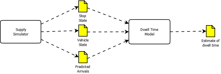
There are three key entities which are defined as inputs to the dwell time model:
- Stop State
- Vehicle State
- Predicted bus arrivals
They are described in more detail below
7.1.1.1 Stop State
A stop state record contains information pertaining to the stopping point. The attributes of this entity are given in the table.
| Name | Description |
|---|---|
| Stop Id | Unique identifier of stop |
| Mode | Indicates the mode of the stop |
| Stop Type | Indicates whether the bus stop is:,Bay bus,On-road,Bus station |
| Stop status | Indication of whether the stop is open or closed.,NB. Sometimes stops can be suspended due to road-works |
| Dwell time model | Reference to the dwell time model to use for this stop. Initially only two types of model will be used: Front door entry: Entry only on front door. Exit at any door. Any door entry: Entry and exit at any door. Such bus stops occur at the border and checkpoints |
| List of passengers at stop | This is a list of passengers at the stop |
7.1.1.2 Vehicle State A vehicle state record contains information about the PT vehicle arriving at the stop and its current state. The attributes of this entity are given in table below.
| Name | Description |
|---|---|
| Vehicle Id | Unique identifier of the bus |
| No levels | Indicates the bus type.,In future the dwell time model may have different models for double deck buses compared to single deck buses |
| No doors | Number of doors on the bus |
| Standing capacity | The maximum number of people allowed to stand on the bus at any one time |
| Seating capacity | The maximum number of people allowed to sit on the bus at any one time |
| Vehicle Line | This is the line of the bus |
| List of stops served | This is a list of stops that are scheduled to be served in the current trip and have not been served yet. Stops are listed in the order that they will be served. |
| Schedule adherence | This indicates the amount of seconds that a bus is ahead of or behind schedule. NB. This can be null if no holding strategy is used |
| Headway Ahead | This indicates the time gap between the current bus and the bus downstream on the same line. NB. This can be null if no holding strategy is used |
| Headway Behind | This indicates the time gap between the current bus and the bus upstream on the same line. NB. This can be null if no holding strategy is used |
| Holding strategy | This indicates the holding strategy of the bus: Schedule adherence, Headway, None. NB. This can be null if no holding strategy is used |
| Line dwell time model | This is an indication of any special dwell time model that should be applied to this bus line.,For example some lines are free to use so passengers can board or alight at any door.,If this is Null then use the dwell time model stated for the stop.,If this is non-null then use the dwell time model specified |
| List of passengers on bus | This is a list of passengers on the bus |
7.1.1.3 Predicted bus arrivals
A predicted bus arrival record contains predictions about future bus arrivals at this stop. This is needed because some travelers may have access to real time bus information and may prefer to wait for another bus even if the bus arriving takes them closer to their destination. The attributes of this entity are given in the following table. The supply system must provide a list of all buses predicted to arrive within the next X minutes where X is configurable and is defaulted to 30 minutes.
| Name | Description |
|---|---|
| Vehicle Id | Unique identifier of the bus |
| Vehicle Line | This is the line of the bus |
| List of stops served | This is a list of stops that are scheduled to be served in the current trip and have not been served yet. Stops are listed in the order that they will be served. |
| Predicted arrival time | This is the absolute time that the bus is predicted to arrive at the bus. |
7.1.2 Outputs
Table below defines the output from the dwell time model.
| Name | Description |
|---|---|
| Stop Id | Unique identifier of stop |
| Vehicle Id | Unique identifier of the bus that the dwell time calculation is for |
| Timestamp | Timestamp that the estimate of dwell time was made at. This uses the simulation time |
| Mode | Indicates the mode of the stop |
| Stop Type | Indicates whether the bus stop is: Bay bus, On-road, Bus station |
| Stop status | Indication,of whether the stop is open or closed. NB. Sometimes stops can be,suspended due to road-works |
| Dwell time model | Reference to the dwell time model to use for this stop. Initially only two types of model will be used: Front door entry: Entry only on front door, Exit at any door. Any door entry: Entry and exit at any door. Such bus stops occur at the border and checkpoints |
| Parking Location | This indicates the location in the stop that the bus will park. Distance is measured from the,front of the bus to the front of the stop.,Refer to section 6.2. |
| Dwell Time | This is the time that the bus will spend stopped at the stop to allow passengers to board and alight the bus |
| Exit Time | This is the time that the bus will spend waiting to exit the bus stop once the dwell time stage has completed.,This time is caused by the bus waiting for a suitable gap in the main traffic stream |
| Departure Time | This is the time that the bus is expected to return to the main traffic stream – i.e. enter segment 2 |
Passengers can arrive at the stopping point by two means:
- From another PT vehicle
- Initial stopping point in trip
In the first case, the passenger arrivals will be determined by the supply simulator. In the second instance where the stopping point is the first one in the trip, the arrival time will be determined by the demand model – refer to the Departure Time Choice Model of section 7 in reference [1].
7.3 Default dwell time model A default dwell time model has already been incorporated into SimMobility and this will initially be used by SimMobility. The dwell time, DT, is given by equations below. It is taken from section 3.4.2 of the Master’s thesis of Oded Cats [10].
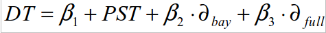
Where:
PST = Passenger Service Time
δbay = Indicates bus stop type: 1 if a bay-type bus stop, 0 otherwise.
δfull = Indicates on-road bus stop type: 1 if an on-road type bus stop, 0 otherwise.
β1, β2, β3 = parameters to be estimated = 0.7, 0.7, 5 respectively
The Passenger Service Time, is given by equation
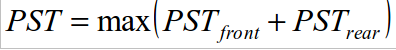
Where PSTfront is the passenger service time at the front door, and PSTrear is the passenger service time at the rear door. They are given by the equations below.
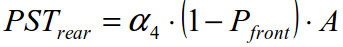
Where: α4 = 1.0 Pfront = Proportion of alighting people who used the front door to exit A = number of passengers alighting at stop

Where:
- α1= alighting passenger service time assuming payment by smart card = 2.1. It should be noted that if passengers are standing in the bus then this value is increased by 0.5.
- α2= boarding passenger service time assuming alighting through rear door = 3.5
- α3= alighting passenger service time assuming payment by smart card = 3.5
- B = number of passengers boarding bus at stop
- CF = indicator of the of crowdedness factor of bus. If passengers have to stand due to there being no available seating then this is 1, otherwise 0.
7.4 Holding strategy
Service quality regulations often require that buses adhere to a schedule or confirm to a certain headway. To ensure that this can happen, a controller at the central depot will often ask individual buisesbuses to wait at a bus stop. This holding strategy can results in buses having additional dwell time above that required to allow all passengers to board and alight.
??? HOLDING STRATEGIES TO BE ELABORATED ON ???
7.5 Differences with SimMobility short term
The key differences between modelling dwell time in mid-term SimMobility (MTS) and short term SimMobility (STS) are given below:
-
In STS dwell time is determined from simulation as it models the movement of each individual passenger onto and off the bus. However in MTS the dwell time is determined from a formula - the number of passengers alighting and boarding is calculated at the instance the bus stops at the stopping point.
-
In MTS only passengers which were at the stop before the bus arrived are able to board the bus. STS allows for “late arrivals” to board the bus.
-
Concerning the passenger route choice, in STS the intended bus line will be given as part of the trip chain.
8 Modelling movement of buses between stops
Sections 6 and 7 have discussed how buses should be modelled at bus stop. However it is important also to model how buses are moved between bus stops. This section describes this.
In the most part the existing concepts to move vehicles on the road network will be used. That is a bus will be treated like any other vehicle on a segment having a queuing part and a free-flow part. However the following modifications will have to be made:
- The PCE (passenger car equivalents) concept is applied when computing density and capacity when buses are added;
- Buses are treated similar to other vehicles in terms of modelling speed: the speed of bus also follows speed-density relationship
- Buses are converted to equivalent number of private cars when computing segment density and receiving capacity of the segment
- Buses consumes additional capacity when passing the boundaries between adjacent segments
- Buses are able to use bus lanes. It should be noted that this functionality to restrict lane usage does NOT yet exist in DynaMIT. The closest similar function or modelling HOV lanes, allows restrictions only at the link level.
- Buses might have a smaller maximum speed than private vehicles. This will be especially relevant for those bus lines which travel on expressways.
NEED TO PROVIDE MORE DETAILS
9 Controller Actions
It is not only the driver which impacts the movement of a public transport vehicle. There are two types of controllers which also have to be included:
-
Service Controller: This will be an agent that is monitoring the overall performance of each bus line, and ensuring that it is being run as desired. In reality this means whether buses are running to schedule and whether the time gap between buses is acceptable
-
Urban Traffic Controller systems: UTC systems can typically give buses priority at signalized junctions.
-
Driver: The driver will choose the actual start time of the vehicle journey. Also the driver of a bus will change during the day as the driver’s schedule differs to the bus schedule.
NEED TO ADD FUNCTIONALITY FOR THE FOLLOWING:
- Controller assigning vehicle to a block
- Controller diverting a vehicle journey
- Controller providing bus priority
- Controller curtailing a vehicle journey
- Controller holding a bus
- Duty changeover
- Decision on exact time to start a vehicle journey
10 Appendix 1: Future issues to resolve
10.1 On-line calibration
On-line calibration is where the simulator is able to correct certain parameters or other attributes dependent on observed real time data.
10.1.1 Data that can be used for on-line calibration of PT
For the existing DynaMIT simulator, aggregated measurements of flow and speed over a certain time period measured at a fixed sensor location are used for this calibration. This data is used as it is commonly collected by transit agencies to monitor the network and control UTC systems.
The type of data that is typically collected for public transport, and in particular buses, is quite different. Data currently collected for PT vehicles is far more disaggregated than that used for monitoring the roads. Real time data that is typically currently available, or likely to be available, within the next 5 years is listed below:
Location of each bus: Modern bus AVL systems report the location of the bus back to a central server at periodic intervals (typically every 30 seconds to 5 minutes). The system will provide a timestamp, and longitude and latitude of the bus. Alternatively the AVL system can provide the time that the bus departed from a given bus stop on route.
Passenger boardings: New ticketing technologies being incorporated in cities such as London, allow passengers to pay for journeys using bank cards. These transactions take place in real time. It will therefore be possible with such systems to capture all origins in near real time. It should be noted that very few cities require passengers to tap out of buses, so in most places the destination of passengers is unknown.
Bus Passenger Counting systems: Increasingly buses have passenger counting systems installed which indicate the number of people on the bus.
10.1.2 How this will be implemented TO BE FINISHED