Math Fourier Epicycles

Fourier epicycles

A chain of circles, each riding the rim of the one before, can draw any closed curve. That is the whole content of the Fourier series of a periodic complex signal, and it is also, almost to the letter, what Greek astronomers did to the planets. View Ptolemy uses the identity twice over: the apparent path of a planet is a slow deferent circle plus a chain of twelve epicycles, and the chain is not invented but computed, by a direct discrete Fourier transform of the last minute of a process's CPU and memory. This page derives the mathematics from the bottom (phasors, the DFT, Parseval, truncation, Gibbs ringing, the sliding window, retrograde loops), says exactly what src/ptolemy.rs and src/simulation.rs do with it, and says what a viewer can and cannot read from the result.

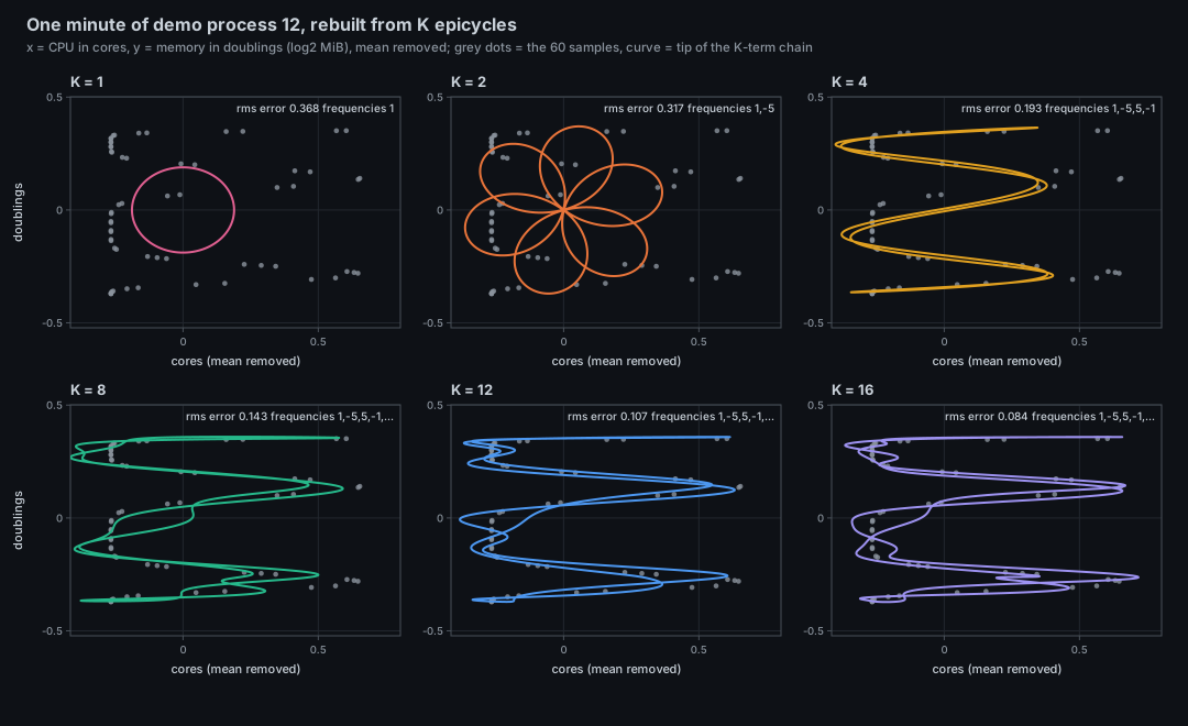
Process 12 of the --demo workload over t = 240 to 299 s, as the view sees it: x is CPU in cores, y is memory in doublings (log2 MiB), mean removed. The grey dots are the sixty samples; the curve is the tip of the K-term chain. Figure script: docs/figures/fourier-epicycle-reconstruction.py.

History

The longer account lives in the repository: docs/theory/ptolemy.md.

Circles first. Greek astronomy was asked to explain the wandering of the planets with uniform circular motion. Eudoxus answered with nested rotating spheres in the 4th century BCE. Apollonius of Perga (about 262 to 190 BCE) is the usual source for the deferent and the epicycle, and for the theorem that an eccentric model and an epicyclic one give the same motion of the Sun. Hipparchus (2nd century BCE) fitted such models to observations of the Sun and Moon.

Ptolemy. Claudius Ptolemy's Mathematical Syntaxis, known by its Arabic title, the Almagest (about 150 CE), is the finished system. For the planets he added the equant, an off-centre point about which the epicycle's centre moves uniformly. It broke the letter of uniform circular motion and was criticised for some fourteen centuries. Nasir al-Din al-Tusi (1247) and Ibn al-Shatir (14th century) repaired it with circles alone; Copernicus (1543) moved the Sun to the middle and still used epicycles, and Kepler's ellipses (1609) removed them. How much Copernicus knew of the Islamic models is debated.

Fourier. Joseph Fourier presented his memoir on heat conduction in 1807 and published Theorie analytique de la chaleur in 1822, arguing that an essentially arbitrary function on an interval can be written as a sum of sines and cosines. The complex form of the statement is the epicycle theorem of section 1. N. R. Hanson (1960) drew the historical moral: an epicyclic system with enough circles can approximate any periodic motion, so the Almagest's long success is no evidence for the heavens being built of circles.

The fast transform. Carl Friedrich Gauss worked out a fast algorithm for the discrete transform around 1805 (the date is presumed) to interpolate the orbits of the asteroids Pallas and Juno from a few observations. He did not publish it; it appeared only in his collected works, and Heideman, Johnson and Burrus drew attention to it in 1984. J. W. Cooley and J. W. Tukey published the algorithm independently in 1965. By Cooley's own later account the occasion was a 1963 meeting of the President's Science Advisory Committee on detecting underground nuclear tests, where Tukey sketched the idea and Richard Garwin, who wanted a fast transform for his own purposes, brought it to Cooley. The Tukey of that meeting also coined the word "bit". Sources differ on what Garwin told Cooley at the time.

Machines. The planetarium projector (Zeiss, 1923) and the orrery before it are mechanical epicycle machines: gears on gears, each a circle on the end of another.

1. Theory: a periodic curve is a sum of rotating vectors

1.1 Phasors

Identify the plane with the complex numbers, so a point is z = x + iy. The function $t \mapsto a e^{i(\omega t + \varphi)}$ is a point moving on a circle of radius |a| = a, with angular velocity $\omega$ (counter-clockwise when $\omega > 0$) and phase $\varphi$ at t = 0. Add a second such term and the sum is a point on a circle whose centre itself moves on a circle: an epicycle. A chain of K terms is

$$ z(t) = \sum_{j=1}^{K} c_j, e^{2\pi i k_j t / T}, \qquad c_j \in \mathbb{C},; k_j \in \mathbb{Z}. $$

The modulus |c_j| is the radius of the j-th circle, $\arg c_j$ is where its radius starts, and k_j is how many turns it makes per period T, clockwise when k_j < 0. Every term has an integer number of turns per period, so the whole chain returns to where it started after T: it draws a closed curve and replays it forever.

1.2 Which circles? The Fourier coefficients

Let z(t) be any T-periodic complex signal (piecewise smooth, say). The exponentials $e_k(t) = e^{2\pi i k t/T}$ are orthonormal for the inner product $\langle f, g\rangle = \frac1T\int_0^T f\bar g,dt$, because for integer $m \ne 0$ the integral of $e^{2\pi i m t/T}$ over a period is zero. Expanding $z = \sum_k c_k e_k$ and taking the inner product with e_l isolates one coefficient:

$$ c_k = \frac{1}{T}\int_0^T z(t), e^{-2\pi i k t/T},dt . $$

That is Fourier's series (Fourier, 1822, for the heat equation; the complex exponential form is a later convenience). The plane curve t -> z(t) and the pair of real signals x(t), y(t) are the same object: a real signal x(t) alone gives $c_{-k} = \overline{c_k}$, two counter-rotating circles whose imaginary parts cancel and whose sum is a point oscillating on a line (a harmonic oscillator is a degenerate ellipse made of two epicycles). A genuinely complex signal breaks that symmetry; the amplitude of c_k against c_{-k} is the eccentricity and the handedness of the ellipse that frequency traces.

1.3 Samples: the discrete transform

isotop does not have a function, it has N = 60 samples z_n = z(nT/N). Define

$$ X_k = \sum_{n=0}^{N-1} z_n, e^{-2\pi i k n/N}, \qquad z_n = \frac1N \sum_{k=0}^{N-1} X_k, e^{2\pi i k n/N}. $$

The inverse holds because $\sum_{n} e^{2\pi i (k-l) n/N} = N\delta_{kl}$ (a geometric series). Comparing with 1.2: the epicycle coefficient is c_k = X_k / N. Two facts matter.

• Aliasing and folding. $e^{2\pi i k n/N}$ and $e^{2\pi i (k-N) n/N}$ agree at every integer n, so k and k - N are the same term on the samples. They differ between samples. The smoothest curve through the samples uses the frequency of smaller magnitude, so a coefficient at index k is assigned the signed frequency k if k < N/2 and k - N otherwise. This is the fold in epicycles() of src/ptolemy.rs. For N = 60 the frequencies run from -30 to +29 turns per window; the -30 term is the Nyquist term and exists only once.
• Trigonometric interpolation. The same formula evaluated at fractional t is a periodic interpolant: it passes through every sample when all N - 1 non-mean terms are kept, and wiggles between them in the least-oscillating way the periodic assumption allows. The view evaluates it at every frame, so it needs no resampling.

The transform assumes the window is one period of a periodic signal. A minute of a process is not periodic; the discontinuity between the last sample and the first is a real feature of the model (section 1.5).

1.4 Parseval, and which K terms are best

The transform is $\sqrt N$ times a unitary matrix, so energy is conserved:

$$ \frac1N\sum_{n} |z_n|^2 = \sum_{k} |c_k|^2 \qquad\text{(Parseval).} $$

Suppose a chain keeps the set S of indices (the mean k = 0 is dropped separately, section 3). Then the mean-square error over the samples is

$$ \frac1N\sum_n \bigl|z_n - \tilde z_n\bigr|^2 = \sum_{k\notin S} |c_k|^2 , $$

with no cross terms because the basis is orthonormal. For a given K the error is smallest when S holds the K largest |c_k|: the error is the total minus $\sum_{S}|c_k|^2$, and a sum of K terms is maximised by the K largest. Greedy selection by amplitude is therefore optimal, not a heuristic, among all K-term sums of these exponentials. That is why epicycles() sorts by |X_k| (ties by index) and truncates.

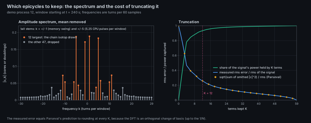
The same window. Left: amplitudes by signed frequency, the twelve the view keeps in orange. Right: the measured rms error at the sixty samples (blue) lies exactly on Parseval's prediction (yellow dots). Twelve terms hold 93.3 % of the signal's power and leave an rms error of 0.258 of the signal's rms. Script: docs/figures/fourier-epicycle-spectrum.py.

In that window the spectrum is not a pair of lines. The demo's CPU wave has a period of $2\pi/0.55 = 11.4$ s, so a 60 s window holds 5.25 cycles. A non-integer number of cycles in a rectangular window spreads each line into the Dirichlet kernel's main lobe and side lobes (spectral leakage), which is why the stems at $\pm 5$ are surrounded by smaller ones and why twelve terms still miss 7 % of the power. The sharp $\sin^4$ pulses add harmonics at about 10.5, 15.8, ... turns per window.

1.5 Gibbs ringing

Where a periodic signal jumps by J, the partial sums of its Fourier series overshoot on each side by about $(\mathrm{Si}(\pi)/\pi - \tfrac12) J \approx 0.0895,J$ however many terms are kept: the Wilbraham-Gibbs phenomenon. The overshoot narrows as K grows but does not shrink. A process whose memory climbs steadily through the whole minute (a leak, a warming cache) has exactly such a jump, at the wrap from the last sample back to the first. The chain that replays it rings on both sides of the wrap.

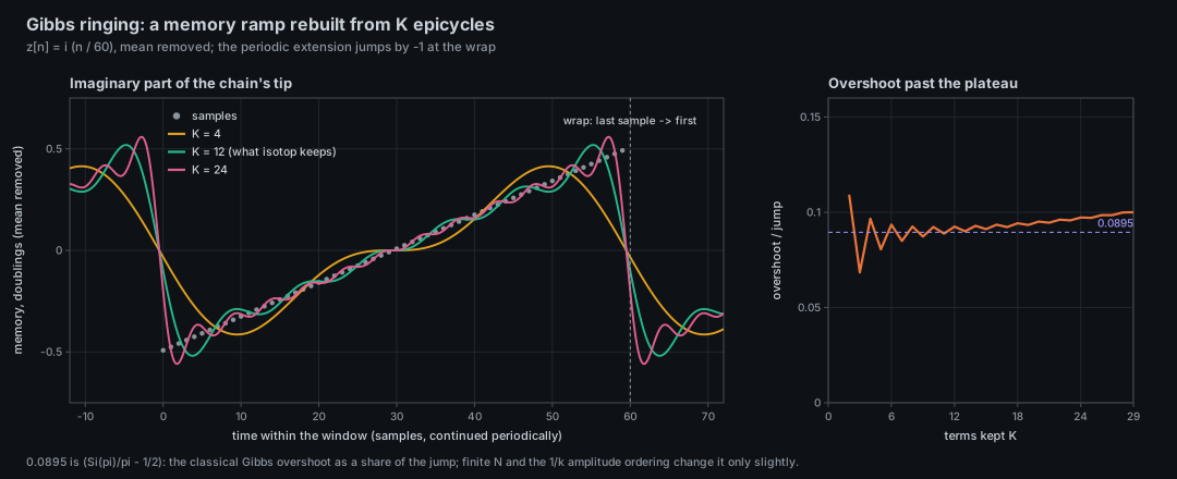
A ramp i n/60, rebuilt with the view's selection rule. The excess over the ideal ramp, as a share of the jump, is about 0.09 for every K from 4 upwards (right; it varies between 0.07 and 0.11 at this N). Script: docs/figures/fourier-epicycle-gibbs.py.

The remedies are standard and absent from isotop: taper the window (Hann, Hamming; Harris 1978 is the survey) so the periodic extension has no jump, weight the coefficients by Fejer or Lanczos sigma factors, or subtract the best straight line before the transform and add it back as a drift. The first costs resolution, the second and third cost fidelity to the measured samples. See section 7.

1.6 A sliding window and why the coefficients hardly move

A new sample arrives each second; the window slides by one. Let X_k be the transform of z_0 ... z_{N-1} and X_k' the transform of z_1 ... z_N. Substituting n -> n - 1 in the sum gives the sliding DFT recurrence (Jacobsen and Lyons, 2003):

$$ X_k' = e^{2\pi i k/N},\bigl(X_k - z_0 + z_N\bigr). $$

The factor $e^{2\pi i k/N}$ is just the rotation of the whole picture by one sample step: replaying the window one step later. If each coefficient is turned back by the phase of the window's first absolute sample number s,

$$ c_k^{(s)} = \frac{X_k}{N}, e^{-2\pi i k s / N}, $$

then $c_k^{(s+1)} = c_k^{(s)} + (z_N - z_0) e^{-2\pi i k s/N}/N$: a slide changes each coefficient by at most $2\max|z|/N$, about 1/30 of the swing. The chain therefore evolves from sample to sample instead of being rebuilt, and the tip can be evaluated at an absolute time t ($e^{2\pi i k t/N}$ with t counted in samples) so that it replays the window in step with the clock. This is the "turned back by its phase at oldest" in the doc comment of epicycles(), and the reason the test dft_reconstruction_equals_the_samples_at_integer_times also checks that sliding a periodic window by one sample leaves the coefficients alone.

1.7 Retrograde motion

Put Earth at the origin and a planet at $p(t) = R e^{i\omega_d t} + r e^{i\omega_e t}$: a deferent of radius R and an epicycle of radius r. Its apparent longitude is $\lambda = \arg p$, and

$$ \frac{d\lambda}{dt} = \frac{\operatorname{Im}\bigl(\bar p, p'\bigr)}{|p|^2}. $$

Retrograde motion is $d\lambda/dt < 0$. Compute $\bar p, p'$ for the two-circle path: with $\alpha = \omega_d t$, $\beta = \omega_e t$,

$$ \operatorname{Im}(\bar p p') = R^2\omega_d + r^2\omega_e + R r(\omega_d + \omega_e)\cos(\beta - \alpha). $$

Its minimum over the relative phase is $R^2\omega_d + r^2\omega_e - Rr(\omega_d + \omega_e) = (R - r)(R\omega_d - r\omega_e)$. For an epicycle smaller than the deferent, r < R, that is negative exactly when

$$ r,\omega_e > R,\omega_d : $$

retrograde motion exists if and only if the epicycle's tip speed exceeds the deferent's speed. Equality is the borderline, a stationary point where the planet halts against the stars (Ptolemy attributes the theorem on stationary points to Apollonius). The same test, on the whole chain, $\operatorname{Im}(\bar p,p') < 0$, is the function retrograde() in src/ptolemy.rs; it needs no assumption about the number of terms.

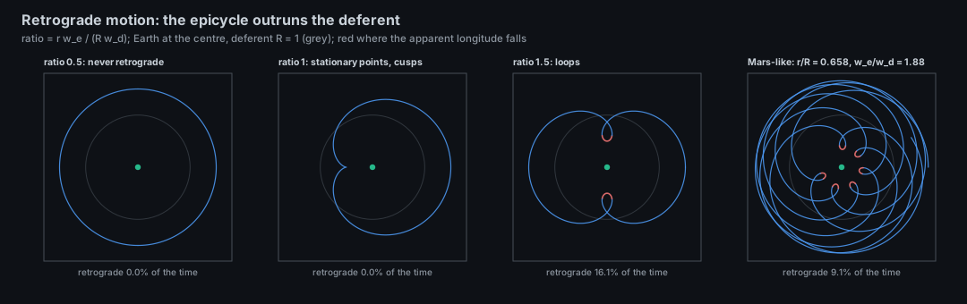
Left to right: ratio $r\omega_e/R\omega_d$ of 0.5 (no retrograde), 1 (cusps), 1.5 (loops) and a Mars-like pair: epicycle-to-deferent ratio 39.5/60 (the Almagest value as it is usually tabulated; unverified here) and $\omega_e/\omega_d = 686.98/365.24$, the sidereal period of Mars over the year, because in Ptolemy's model of a superior planet the epicycle's radius to the planet stays parallel to the direction of the mean Sun. The pure circles-only model spends 9.1 % of the time in retrograde, 71 days of the 780-day synodic cycle; the real sky gives roughly two to two and a half months. Script: docs/figures/fourier-epicycle-retrograde.py.

2. How isotop's geometry differs from Ptolemy's

(The history is above.) isotop's geometry is the uncomplicated one: Earth at the centre of every deferent, uniform angular speed about that centre (no equant, no eccentric), and a chain of epicycles of arbitrary number whose radii and phases are measured rather than fitted to the sky. A uniform deferent plus a chain of epicycles is exactly a Fourier series with one extra low-frequency term (the deferent itself), which is Hanson's point.

The same lesson is the folk theorem about overfitting: "with four parameters I can fit an elephant, and with five I can make him wiggle his trunk", a remark attributed to von Neumann (reported by Dyson, 2004). Mayer, Khairy and Howard (2010) took it literally and drew an elephant with a Fourier series of four complex parameters. Twelve complex epicycles are three times that budget, and the view makes no claim about elephants.

3. What the code does

Step	What happens	Where
Signal	The last SERIES = 60 samples of the shared history: z[n] = cpu / 100 + i * log2(max(MiB, 1)), a sample before a process's first held at its first reading and a gap held at the last reading; then the mean over the window subtracted	signal(), history::SERIES
Transform	The direct, O(N^2), f64-accumulating dft(), forward sign exp(-2 pi i k n / N), no scaling. N = 60 is not a power of two, so the radix-2 fft() in the same file is not used	simulation::dft
Selection	Indices 1 .. N-1 sorted by |X_k| descending (ties by index), the first TERMS = 12 kept, the mean (k = 0) dropped: it is the planet's place on the deferent	epicycles()
Folding	Signed frequency k if k < N/2, else k - N, in turns per REPLAY = 60 s	epicycles()
Coefficient	X_k / N times exp(-2 pi i (k * oldest mod N) / N) with oldest the absolute number of the window's first sample (the sliding-window correction of 1.6)	epicycles()
Scale	One global gain: with T = K * sum |c|, gain = K L tanh(T / L) / T, K = GAIN = 0.085 * 40 = 3.4 world units per core or doubling and L = REACH = 0.19 * 40 = 7.6	scaled()
Replay	The tip is sum c_j exp(2 pi i f_j t / 60 s) at scene time t: the minute replays once a minute, whatever --sample-ms	chain(), rotor()
Easing	When a sample arrives, coefficients ease from their current value to the new target with a smoothstep over the measured sample interval, clamped to 0.1 to 10 s; a term that left the twelve eases to nothing	Planet::retarget, EASE
Retrograde	Im(conj(p) p') < 0 with p the deferent point plus the chain and p' the sum of both velocities	retrograde(), chain_velocity()

The gain is worth a line. With T = K * sum of the radii in cores and doublings, the scaled radii add up to exactly $L\tanh(T/L)$: linear for small $T$ (a process that barely varies gets $3.4$ units per core or doubling) and saturating at $L = 7.6$ units, however wild the process. A process whose radii sum to 1 gets a chain 3.2 units long; to 2, 5.4; to 4, 7.2; to 8, 7.6. The scale is the same for every planet so amplitudes remain comparable between planets, but it is not comparable between a core and a doubling, which View Ptolemy takes up.

Every sphere's deferent is larger than the whole chain. The smallest sphere, the Moon's, has radius 0.245 * 40 = 9.8 against a maximum chain length of 7.6, so the r < R case of 1.7 always applies and retrograde means exactly "the tip speed beats the deferent's speed". The periods follow Kepler's third law, T = 1200 s (r / r_Saturn)^{1.5}, and the speeds are far below those of the epicycles:

Sphere	Radius (units)	Deferent period	Deferent speed	Smallest k = 1 radius that outruns it
Moon	9.8	3.7 min	0.278 u/s	2.65
Mercury	13.2	5.8 min	0.239 u/s	2.28
Venus	16.6	8.2 min	0.213 u/s	2.04
Sun	20.0	10.8 min	0.194 u/s	1.86
Mars	23.4	13.6 min	0.180 u/s	1.72
Jupiter	26.8	16.7 min	0.168 u/s	1.60
Saturn	30.2	20.0 min	0.158 u/s	1.51

(Computed from RADII, SKY = 40, OUTER_PERIOD = 1200; an epicycle of radius $\rho$ and frequency k has tip speed $2\pi k\rho/60$.) A k = 5 term, the demo's CPU pulse, outruns a deferent once it is 0.3 units wide (Saturn's sphere) to 0.5 units wide (the Moon's), so in practice every planet is in retrograde for a large share of the time, unlike the real sky where retrograde loops are rare events of a few weeks. The red trails of View Ptolemy are the common case, not the exception.

4. Reading the picture

• Measured. The coefficients, the radii and the handedness of the epicycles are the best K-term description of the last 60 samples, to the rms error Parseval gives (section 1.4; for the demo process of the figures, 0.107 against a signal rms of 0.415 at K = 12). The tip, evaluated at the sample times, is the process's own (cpu, memory) to that accuracy.
• Derived. Which terms are drawn (the twelve largest), the single global gain, and which stretch of the trail is red are computed, not measured.
• Decorative. The deferent's period (Kepler's law applied to a made-up radius) and the sphere names are decoration; the planet's position on its deferent is a hash of the identity plus uniform motion and carries no information.
• Handedness is information. The real axis is CPU and the imaginary axis is memory. A term $c e^{+i\omega t}$ has $x = |c|\cos(\omega t + \varphi)$, $y = |c|\sin(\omega t + \varphi)$: the memory lags the CPU by a quarter period when the epicycle turns counter-clockwise, and leads it when it turns clockwise. A flat ellipse is CPU and memory in phase, or one of them not varying.
• Invisible. Anything faster than the sample interval (Nyquist, 0.5 cycles per sample), anything slower than the window, and the 47 smaller terms. A process whose CPU pulses are narrower than a sample is aliased to a low frequency before the transform sees it.
• The wrap is not a feature of the process. The snap from the end of the minute back to its start, and the ringing next to it (section 1.5), belong to the periodic assumption.

5. Try it

# Needs a full 60-sample window: the demo's reference time for this view is 300 s.
./target/release/isotop --demo --view ptolemy --time 300 --width 1600 --output /tmp/ptolemy.png
python3 docs/figures/fourier-epicycle-reconstruction.py   # rewrites the figure from the maths above

Live, press v and pick ptolemy (or --view ptolemy); until 30 samples exist the legend reads "the heavens are still forming". Select a planet to read its sphere and epicycle count in the popup.

6. Where in the code

• src/simulation.rs: Complex, dft, fft, inverse_fft, smoothstep. The fft is radix-2 and panics for other lengths; dft accepts any.
• src/ptolemy.rs: signal, epicycles, scaled, chain, chain_velocity, rotor, retrograde, Planet::retarget, Deferent; constants TERMS, GAIN, REACH, REPLAY, RADII, OUTER_PERIOD, EASE.
• src/history.rs: SERIES, History::recent.
• Tests: dft_reconstruction_equals_the_samples_at_integer_times, a_planet_whose_epicycle_outruns_its_deferent_is_in_retrograde_and_a_slow_one_is_not.
• Figure scripts: docs/figures/fourier-epicycle-*.py (with epicycle_w6.py and svgkit_w6.py).

7. Variations and open questions

1. Window the minute. Multiply the window by a Hann taper before the transform. Gibbs ringing at the wrap should vanish, at the cost of a resolution loss of about two bins. Does the tip still pass through the latest sample, which matters when a viewer wants "where is it now"?
2. Detrend, then restore. Fit and remove a line; carry the slope as a drift of the whole chain. A leaking process would then draw a clean spiral instead of a ringing loop.
3. Real frequency estimation. Zero-pad to 128 and use the in-tree radix-2 fft to sharpen the peaks, then fit each peak's true frequency by interpolation. The chain would no longer be periodic in 60 s.
4. Non-1 Hz sampling. The phase correction treats the absolute sample number as time in seconds. With --sample-ms 500 the window is still replayed in 60 s, but a slide of one sample then shifts the replayed curve by half a sample step (an analysis from the code, not a tested behaviour); a clock in sample units would remove it.
5. Per-term sign. Colour clockwise and counter-clockwise epicycles differently so that "memory leads CPU" is visible without reading the rotation.
6. Equant. Add a true Ptolemaic equant to the deferent and ask whether the retrograde statistics of the demo change.

References

• J. B. J. Fourier, Theorie analytique de la chaleur (Paris, 1822).
• M. T. Heideman, D. H. Johnson and C. S. Burrus, "Gauss and the history of the fast Fourier transform", IEEE ASSP Magazine 1(4) (1984), 14-21.
• J. W. Cooley and J. W. Tukey, "An algorithm for the machine calculation of complex Fourier series", Mathematics of Computation 19 (1965), 297-301.
• F. J. Harris, "On the use of windows for harmonic analysis with the discrete Fourier transform", Proceedings of the IEEE 66 (1978), 51-83.
• E. Jacobsen and R. Lyons, "The sliding DFT", IEEE Signal Processing Magazine 20(2) (2003), 74-80.
• H. Wilbraham, "On a certain periodic function", Cambridge and Dublin Mathematical Journal 3 (1848), 198-201; E. Hewitt and R. E. Hewitt, "The Gibbs-Wilbraham phenomenon: an episode in Fourier analysis", Archive for History of Exact Sciences 21 (1979), 129-160.
• N. R. Hanson, "The mathematical power of epicyclical astronomy", Isis 51 (1960), 150-158.
• G. J. Toomer (transl.), Ptolemy's Almagest (London: Duckworth, 1984); O. Neugebauer, A History of Ancient Mathematical Astronomy (Springer, 1975).
• F. Dyson, "A meeting with Enrico Fermi", Nature 427 (2004), 297.
• J. Mayer, K. Khairy and J. Howard, "Drawing an elephant with four complex parameters", American Journal of Physics 78 (2010), 648-649.
• See also View Ptolemy, Theory History, Theory Simulation Toolkit and Math Stellar Photometry.