Math Spatial Hashing

Math: Spatial hashing

How do you find the neighbours of a point among ten thousand others without comparing it with all ten thousand? Cut space into equal cells, file each point under its cell, and look only in the cells the question can reach. This page works out the cost of that idea (how many cells, how many distance tests, what cell size to choose), proves that the shell search for the $k$ nearest neighbours in SpatialHash3::nearest is exact, says where it degrades, and compares it with trees. Every operation count in it is a count, not a timing, and the counts were obtained two ways: by instrumenting a copy of the shipped Rust and by an independent Python port that gave identical numbers.

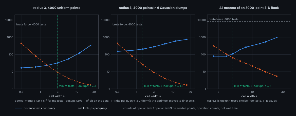
Distance tests (solid) and cell lookups (dashed) per query against cell size. Left: radius queries of 3 units in 4 000 uniform points. Middle: the same radius in 4 000 points in six Gaussian clumps. Right: the 22 nearest of 8 000 flock points in 3-D. Brute force is the horizontal line. The model curves of section 2 sit on the measured points.

History

The idea of binning points into equal cells is older than the word "hash" in this sense. Molecular dynamics met the problem first: every one of $n$ particles interacting through a short-range force needs its neighbours, and $n^2$ tests were unaffordable in the 1960s. Loup Verlet's 1967 paper on Lennard-Jones fluids (Physical Review 159, 98-103) introduced the neighbour list that bears his name, a per-particle list refreshed every few steps. Cell methods, which restrict the search to a particle's own cell and its 26 neighbours, appear in the same literature a few years on; Quentrec and Brot's 1973 note in the Journal of Computational Physics is often cited for them, though this page did not check what it proposed. Tree structures answered the same question for scattered data: Bentley's $k$-d tree (1975), the best-match search of Friedman, Bentley and Finkel (1977) and Meagher's octree encoding (1982) are the ones section 5 compares.

Hashing the cell, rather than allocating a dense array of them, belongs to computer graphics. Matthias Teschner, Bruno Heidelberger, Matthias Mueller, Danat Pomeranets and Markus Gross, at ETH Zurich, presented "Optimized spatial hashing for collision detection of deformable objects" at Vision, Modeling, and Visualization 2003 in Munich (proceedings pp. 47-54). They compressed a potentially infinite regular grid into a finite table with a hash function that does not map cells uniquely, and reported real-time collision and self-collision detection for scenes of up to 20 000 tetrahedra. Their hash multiplies the three integer cell coordinates by the primes 73 856 093, 19 349 663 and 83 492 791 and takes the exclusive-or; the three numbers have since been copied into so many codebases that they behave as folk constants. Ericson's Real-Time Collision Detection (2005) put grids and hashed grids into the standard textbook form.

isotop does not use that hash. It keys cells on the exact integer triple, so distant cells never share a key (section 5). The k-nearest shell search of section 3 is a plain expanding-ring search with an exactness proof, not a result from this literature.

1. The problem

Given $n$ points $p_1,\dots,p_n\in\mathbb R^d$ and a query point $x$, answer one of

• radius query: all $i$ with $\lVert p_i-x\rVert<r$;
• $k$-nearest: the $k$ indices with the smallest $\lVert p_i-x\rVert$.

Brute force is $n$ distance evaluations per query, $n^2$ for all-pairs. For a flocking simulation (every bird asks for its neighbours every step) with $n=8000$, that is $6.4\times10^7$ squared distances per step. The grid makes the cost depend on the answer instead of on $n$.

2. Theory: the uniform grid

2.1 The structure

Choose a cell width $s$. The cell of a point is $c(p)=\lfloor p/s\rfloor$ componentwise. Store the points in one flat array sorted by cell, plus a map from cell to the range of the array it occupies.

• Build: one sort of $n$ indices by (cell key, index), $O(n\log n)$ (a counting sort over a bounded domain would give $O(n)$; the code sorts, so that a cell lists its points in ascending index order, which makes results deterministic). The map is then filled in one pass over the runs of equal keys.
• Rebuild each step: the same buffers are reused, so a steady point count allocates nothing (test rebuild_at_a_steady_point_count_keeps_its_buffers). There is no incremental update: a moving population is simply rebuilt.

2.2 Radius queries: how many cells, how many points

A radius query for $x$ must visit every cell that the cube $[x-r,x+r]^d$ overlaps. Along one axis that is $\lfloor(x+r)/s\rfloor-\lfloor(x-r)/s\rfloor+1$ cells. An interval of length $L=2r$ at a uniformly random offset overlaps $L/s+1$ cells on average: it crosses $L/s$ cell boundaries in expectation and always touches the cell it starts in. So the expected number of cell lookups is

$$ \mathbb E[\text{lookups}]=\Bigl(\frac{2r}{s}+1\Bigr)^{d}. $$

When $2r/s$ is an integer the count is exactly that for almost every $x$.

With uniform density $\rho$ (points per unit volume), a cell holds $\rho s^d$ points, so the distance tests number

$$ \mathbb E[\text{tests}]=\rho s^d\Bigl(\frac{2r}{s}+1\Bigr)^{d}=\rho,(2r+s)^{d}, $$

of which the true neighbours are $\rho V_d r^d$ (with $V_d$ the volume of the unit ball: $\pi$, $4\pi/3$). The precision of the grid, hits per test, is $V_d r^d/(2r+s)^d=V_d/(2+u)^d$, with $u=s/r$. In two dimensions, $u=1$ gives $\pi/9=0.35$; $u=\tfrac12$ gives $\pi/6.25=0.50$; the limit $u\to0$ gives $\pi/4=0.785$, the share of the query square occupied by the query disc. The square, not the disc, is what a grid visits; that is the floor.

2.3 Choosing the cell width

Cost has two parts that pull in opposite directions: lookups are cheap in operations but cost a hash probe (weight $a$), tests cost a few flops (weight $b$). With $m=\rho r^d$ (expected points in a cube of side $r$):

$$ C(u)=a\Bigl(\frac2u+1\Bigr)^{d}+b,m,(2+u)^{d}=(2+u)^d\Bigl(\frac{a}{u^{d}}+b,m\Bigr). $$

Setting $C'(u)=0$:

$$ d(2+u)^{d-1}\Bigl(\frac a{u^d}+bm\Bigr)-d,a,\frac{(2+u)^d}{u^{d+1}}=0 ;\Longrightarrow; bm=\frac{2a}{u^{d+1}} ;\Longrightarrow; u^*=\Bigl(\frac{2a}{b,m}\Bigr)^{!1/(d+1)} . $$

So the best cell is $s^=r,(2a/bm)^{1/(d+1)}$: finer when the data are denser ($m$ large) and coarser when lookups are dear. It is a weak dependence (the $d+1$-th root), so a cell width of the order of the query radius is within a small factor of optimal over a wide range of densities, and the cost near the optimum is flat. With $a=b$, $d=2$ and $\rho=0.4$, $r=3$ ($m=3.6$): $u^=(2/3.6)^{1/3}=0.82$.

2.4 Measured, against the model

Counts per query for $n=4000$ points, uniform in a $100\times100$ square from Rng::new(7) ($\rho=0.4$), radius $r=3$, for the shipped SpatialHash (instrumented copy of simulation.rs) and my independent port:

$s$	$u=s/r$	lookups, model $(2/u+1)^2$	lookups, measured	tests, model $\rho(2r+s)^2$	tests, measured	hits
0.3	0.1	441	441.00	15.9	16.50	12.12
0.75	0.25	81	81.00	18.3	18.75	12.12
1.5	0.5	25	25.00	22.5	22.79	12.12
3	1	9	9.00	32.4	32.00	12.12
6	2	4	4.00	57.6	55.23	12.12
12	4	2.25	2.33	129.6	122.19	12.12
24	8	1.56	1.65	360	333.00	12.12

Brute force is 4 000 tests per query. At $u=1$ the grid does 41 operations (9 lookups and 32 tests), a hundredth of the work. The lookup model is exact at integer $2r/s$; the tests differ by edge effects (the square is clipped by the domain edge at large $s$), and the expected hits $\rho\pi r^2+1=12.3$ (the query point itself is a hit) is reduced to 12.12 by the same edge effect. Coop's cell is its interaction radius, SpatialHash::new(NEIGHBOURHOOD) with NEIGHBOURHOOD = 4.0, which is $u=1$: nine lookups per bird.

3. $k$-nearest by growing shells

A $k$-nearest query has no radius to start from. SpatialHash3::nearest(point, k, out) finds one by visiting shells of cells around the query cell $q=c(p)$: shell $R$ is the set of cells at Chebyshev distance exactly $R$ from $q$ (the surface of a cube of side $2R+1$), $R=0,1,2,\dots$

3.1 The stopping rule and why the result is exact

Let $C_R$ be the cube of cells with Chebyshev distance at most $R$ from $q$, the union of shells $0..R$. Let

$$ \delta_R=\min_{\text{axes }a}\ \min\bigl(p_a-(q_a-R)s,\ (q_a+R+1)s-p_a\bigr) $$

be the distance from $p$ to the nearest face of $C_R$. Since $p$ lies inside cell $q$, $\delta_R\ge Rs$.

Claim. After examining all points in $C_R$, if at least $k$ candidates are held and the $k$-th smallest of their distances satisfies $d_k\le\delta_R$, then the $k$ best candidates are the $k$ nearest points of the whole set, with ties resolved by index as brute force would.

Proof sketch. A point not in $C_R$ lies in a cell outside the cube, so at least one of its coordinates is beyond a face of the cube while $p$ is inside it; its distance to $p$ is therefore at least the distance from $p$ to that face, at least $\delta_R$. Hence every unexamined point is at distance $\ge\delta_R\ge d_k$: none can displace the current $k$-th candidate. The candidates within $C_R$ include every point with distance $<\delta_R$ (because such a point is inside $C_R$), so among the points of the set the $k$ smallest distances are the $k$ smallest among candidates. For ties, the code requires the strict margin $d_k(1+10^{-6})\le\delta_R$, so an unexamined point can never tie with the $k$-th candidate; ties among examined candidates are broken by index, as the brute-force reference does. $\square$

Termination, and the cost bound. Because the ball of radius $Rs$ about $p$ lies inside $C_R$, the candidate set after shell $R$ contains every point within $Rs$ of $p$. Let $d_k^\star$ be the true $k$-th distance. Once $Rs\ge d_k^\star$ the $k$ true nearest are all candidates, the candidate $k$-th distance equals $d_k^\star\le Rs\le\delta_R$, and the rule fires. So the search stops by shell

$$ R_{\rm stop}\le\Bigl\lceil\frac{d_k^\star}{s}\Bigr\rceil , $$

visiting at most $(2R_{\rm stop}+1)^3$ cells. If $s\ge d_k^\star$, then $R_{\rm stop}\le1$ and at most 27 cells are visited. This is the sizing rule in the doc comment: "choose a cell a little wider than the typical distance to the $k$-th neighbour". For uniform density $\rho$ the expected $k$-th distance is $d_k=\bigl(3k/(4\pi\rho)\bigr)^{1/3}$ (the ball that contains $k$ points has volume $k/\rho$), so with $s=d_k$ the search examines about $27\rho s^3=27\cdot3k/4\pi=6.4,k$ points for the $k$ it returns: $142$ for $k=22$.

Fallback. If the cube of the next shell would hold more cells than there are points ($(2R+1)^3>n$), the search stops growing and scans all $n$ points: no worse than brute force. So the cost is $\min(n,\ \text{shells})$, never more than $n$ plus the shells already walked.

3.2 The per-cell pruning, and why it keeps exactness

Within a shell most cells are far from $p$ once $d_k$ is known. visit_shell computes, for a cell offset $(dx,dy,dz)$, the squared distance from $p$ to the nearest point of that cell, $\sum_a g_a(\text{offset}_a)^2$ with $g_a=0$ for offset 0 and otherwise the gap to the cell's near face, and skips the cell if it exceeds the squared current $k$-th distance. A skipped cell cannot hold a point nearer than the $k$-th candidate, so skipping changes the cost but not the result. In f32 the code widens every comparison by $10^{-6}$ relative (and the face distance by a slack of $4\times10^{-7}$ of the coordinate magnitude) so that a point a few ulps over a cell boundary, or a distance rounded down, can never be lost.

3.3 Measured: 22 nearest of an 8 000-point flock

The flock is the one of the unit test timing_nearest_22_of_8000_flock_points_and_fft_1024: 11 Gaussian clumps (centres $\sigma=18$, birds $\sigma=14$ about their clump, the whole thing 60 up), from Rng::new(51). Per query, over all 8 000 queries (each query point is itself stored, so the query is "the point plus its 21 nearest"):

cell $s$	distance tests	cell lookups	tests + lookups
2.5	79.27	318.69	398.0
4	78.66	102.44	181.1
5	107.61	62.87	170.5
6.5 (the test's choice)	190.32	40.79	231.1
8	265.85	30.22	296.1
10	327.94	21.29	349.2
13	421.80	13.83	435.6
16	534.95	9.67	544.6
24	961.79	5.43	967.2

Brute force would be 8 000. At 6.5 the grid does a forty-second of the distance work. All nine rows return the same neighbours (the checksum of the last-neighbour index over the 8 000 queries is identical, $32,157,502$, for every cell size, as exactness predicts). The 22nd-neighbour distance of this flock has median 6.1, mean 7.0, 10th percentile 4.4, 90th percentile 10.6 and maximum 34.4 (the doc comment says "about 5 units"; the median here is 6.1, so the cell of 6.5 is a little more than one median distance wide and the fraction of queries needing a second shell is large).

Two lessons. First, equal weights put the optimum at 5; a lookup is a hash probe and a test is three multiplies, so the true optimum sits to the right of this table's, where the author put it. Second, the per-query cost is heavy-tailed: at $s=6.5$ the distance tests per query have median 163, 90th percentile 354, maximum 457, but cell lookups have median 27, 90th percentile 61, 99th percentile 259 and maximum 1 331: an outlier bird, 34 units from its 22nd neighbour, walks five shells, the whole $11\times11\times11$ block, because with fewer than 22 candidates nothing can be pruned. One cell width cannot be right for a dense core and a sparse halo; see the next section.

4. Degenerate distributions

• Coincident points. All $n$ points in one cell: a query visits one cell and tests all $n$ (measured: 1 lookup, 2 000 tests for 2 000 coincident points). It is brute force plus one probe. For radius queries the work is output-sensitive (all $n$ really are neighbours); for $k$-nearest it is the worst case. The test spatial_hash_handles_empty_and_coincident_points covers correctness, and the nearest test with 30 coincident points checks that the index breaks the tie.
• Clustered data. Density varies by orders of magnitude, so any single $s$ is wrong somewhere: too coarse in the core (many tests per hit), too fine in the halo (many empty lookups). The middle panel of the figure: six Gaussian clumps, $\sigma=4$, radius 3, give 111 hits per query (against 12 for uniform); tests + lookups is smallest at $s=1.5$ ($u=0.5$: 205 + 25 = 230) rather than at $s=3$ (276 + 9 = 285). This is the $u^*\propto m^{-1/(d+1)}$ of section 2.3 with a larger effective $m$.
• Query radius much larger than the cell. The visited box has $(2r/s+1)^d$ cells, which can exceed $n$; neighbours then scans all points (cells > points.len()), so the cost is $\min(\text{cells},n)$-ish. The product of spans can overflow, so it is computed saturating in i64.
• Extreme or non-finite coordinates. Cell coordinates are i32, produced by a float-to-int cast that saturates and maps NaN to 0, so every input yields a cell. SpatialHash3 additionally records gridded = false if any point is non-finite or has a cell coordinate beyond $\pm2^{30}$ (CELL_LIMIT). A grid with gridded = false, a query point with a non-finite coordinate, or a query cell beyond the limit answers by scanning every point, which is correct and slow (tests nearest_scans_every_point_for_extreme_or_non_finite_coordinates, a_radius_beyond_the_cell_range_scans_every_point_without_overflowing).
• Flat data. If all $z$ are equal the 3-D grid is a slab: occupied cells are a 2-D set, but the shell loops still enumerate all $(2R+1)^3$ offsets; the per-cell pruning skips most of them by their $z$ gap, at the price of one comparison each.
• Radius query in f32. The proof of a radius query is two lines in real arithmetic: a point at distance $<r$ has every coordinate within $r$ of $x$, so its cell index is between the cells of $x\pm r$ by monotonicity of $\lfloor\cdot\rfloor$. In f32 the bounds $x\pm r$ are rounded, so a point whose distance rounds to just under $r$ in the test could sit one ulp outside the rounded box. neighbours does not widen its box (the shell search does, as above); the tests compare with brute force on seeded sets and find no difference, and the band is of relative width $10^{-7}$.

5. Grid versus trees

	build	radius query	$k$-nearest	adapts to density	updates
uniform grid (here)	$O(n\log n)$ sort, $O(n)$ by counting	$O\bigl((2r/s+1)^d+\rho(2r+s)^d\bigr)$	$\sim27,\rho s^3$ tests if $s\ge d_k$	no: one scale	rebuild
$k$-d tree (Bentley 1975)	$O(n\log n)$	$O(n^{1-1/d}+\text{hits})$ worst, $O(\log n+\text{hits})$ typical	$O(\log n+k)$ expected (Friedman, Bentley and Finkel 1977)	yes: splits at the median	rebuild or lazy
octree / quadtree (Meagher 1982)	$O(n\log n)$	$O(\log n+\text{hits})$ for bounded depth	like $k$-d	yes: subdivides where dense	local, cheap
BVH / R-tree	$O(n\log n)$	$O(\log n+\text{hits})$	similar	yes	refit
hierarchical grids	$O(n\log n)$	one grid per scale	per scale	partly	rebuild

A grid wins when (a) the query scale is known and roughly uniform ($r$ is an interaction radius), (b) the data are rebuilt every step anyway, (c) the working set fits in cache, so that probing a cell is a few adjacent array reads, and (d) simplicity matters. Trees win on strongly clustered data or a wide spread of query scales. isotop's populations (192 to 10 000 processes; 8 000 birds in the Murmuration flock (BIRD_CAP)) sit squarely in the grid's regime. The HashMap from cell to range (instead of a dense 3-D array) is what lets the domain be unbounded: only occupied cells exist, and a key is the cell's integer triple (SpatialHash packs two i32 into one u64; SpatialHash3 keys on [i32; 3] with its own multiply-and-fold hasher, because the default SipHash "cost a k-nearest query about as much as the distances it computes"). For the same reason a Gaussian flock never needs the empty space between clumps, which a dense grid would allocate.

Teschner et al. (2003) analyse the same structure as a hash table of cells for collision detection (they hash cell coordinates into a table smaller than the domain and accept collisions between distant cells); isotop avoids false sharing by keying on the exact cell triple instead.

6. How isotop realises it

• SpatialHash (2-D, radius only) has one production user: Coop's Vicsek flocks (SpatialHash::new(NEIGHBOURHOOD), NEIGHBOURHOOD = 4.0 world units, rebuilt per fixed step; see Flocking).
• SpatialHash3 (3-D, radius and exact $k$-nearest) has one production user, the Murmuration view (src/murmuration.rs): Flock calls nearest once per bird per fixed step, asking for FAR_NEIGHBOURS + 1 = 22 points (the bird and its 21 nearest), and takes the seven nearest of them for alignment. Its Grid::adapt rebuilds the hash with a cell as wide as the mean distance of a bird to its 21st neighbour whenever that is more than a quarter off the cell it has, clamped to CELL_RANGE = (1.0, 8.0) from a start of CELL = 2.0; the sizing rule of section 3.1 is therefore applied at run time. The 3-D radius query neighbours is still used only by tests.
• Results are deterministic (sorted by index, or by distance then index) and independent of hash order, which keeps the frames reproducible (Determinism).
• The measured timing (not a count): the ignored test asserts that 22-nearest queries for 8 000 points take under 10 ms in release.

7. Reproducing the counts

The counts above were produced twice. (1) A copy of src/simulation.rs outside the repository, with atomic counters added to the distance and lookup sites, driven by a small program that reads a point file; (2) a Python port of the algorithm (docs/figures/hashing-op-counts.py carries the version that regenerates the figure; it contains the port of Rng and of both queries). On the same point files the two agree to the printed digits in every row of the tables of sections 2.4 and 3.3. To regenerate the figure:

python3 docs/figures/hashing-op-counts.py

8. Variations and open questions

• Adaptive cell width, beyond the mean. Murmuration already adapts $s$ to the mean 21st-neighbour distance (Grid::adapt). The heavy tail of section 3.3 argues for a two-level grid (coarse cells, subdivided where occupied beyond a threshold).
• Counting sort. Replace the $O(n\log n)$ sort by a two-pass counting sort over occupied cells. The determinism requirement (ascending index inside a cell) is met by a stable scatter.
• Morton order. Sort by the interleaved bits of the cell coordinates so that spatially near cells are near in memory; the shell loops then stream.
• Exact count of the sphere-pruned cells. Derive the expected number of cells that survive the squared_gap test as a function of $s/d_k$ and compare with the 40.8 lookups at 6.5.
• A radius-widening neighbours. Mirror the shell search's $10^{-6}$ slack in the radius box so that the two APIs share one rounding guarantee.

9. Where in the code

• src/simulation.rs: SpatialHash (new, rebuild, neighbours), SpatialHash3 (rebuild, neighbours, nearest, visit_shell, face_distance, width), Cell, CellHasher, CELL_LIMIT, rank, closer; the tests spatial_hash_finds_exactly_the_points_brute_force_finds, nearest_finds_exactly_what_brute_force_finds, neighbours_in_3d_finds_exactly_what_brute_force_finds, timing_nearest_22_of_8000_flock_points_and_fft_1024.
• src/coop/sim.rs: the one user of SpatialHash.
• src/murmuration.rs: the one user of SpatialHash3 (Flock, Grid::adapt).
• docs/mockups/code/murmuration.py: the flock the tests are scaled from.

10. References

• Bentley, J. L. 1975. "Multidimensional binary search trees used for associative searching." Communications of the ACM 18(9): 509-517.
• Bentley, J. L. and Friedman, J. H. 1979. "Data structures for range searching." ACM Computing Surveys 11(4): 397-409.
• Friedman, J. H., Bentley, J. L. and Finkel, R. A. 1977. "An algorithm for finding best matches in logarithmic expected time." ACM Transactions on Mathematical Software 3(3): 209-226.
• Meagher, D. 1982. "Geometric modeling using octree encoding." Computer Graphics and Image Processing 19(2): 129-147.
• Teschner, M., Heidelberger, B., Mueller, M., Pomeranets, D. and Gross, M. 2003. "Optimized spatial hashing for collision detection of deformable objects." Vision, Modeling, and Visualization (VMV) 2003.
• Verlet, L. 1967. "Computer 'experiments' on classical fluids. I. Thermodynamical properties of Lennard-Jones molecules." Physical Review 159(1): 98-103.
• Ericson, C. 2005. Real-Time Collision Detection. Morgan Kaufmann.
• Samet, H. 2006. Foundations of Multidimensional and Metric Data Structures. Morgan Kaufmann.