Planned Morph

Planned: Morph

Planned, not yet implemented. Specified in docs/briefs/views-2026-10.md and tracked in issue #50.

A glossy embossed dish of Gray-Scott reaction-diffusion patterns, seen isometrically, in which every process owns a patch and the patch's morphology reads the process's CPU: sparse drifting spots when idle, solitons under light work, fingerprints, mazes, then honeycomb holes, and boiling turbulence on several cores. Memory sets how much dish a process claims; an exited process stops being fed and its pattern starves to dark. This page is the design of that view. The mathematics lives in Math-Reaction-Diffusion; here the question is what the design does with it and what a viewer may honestly infer.

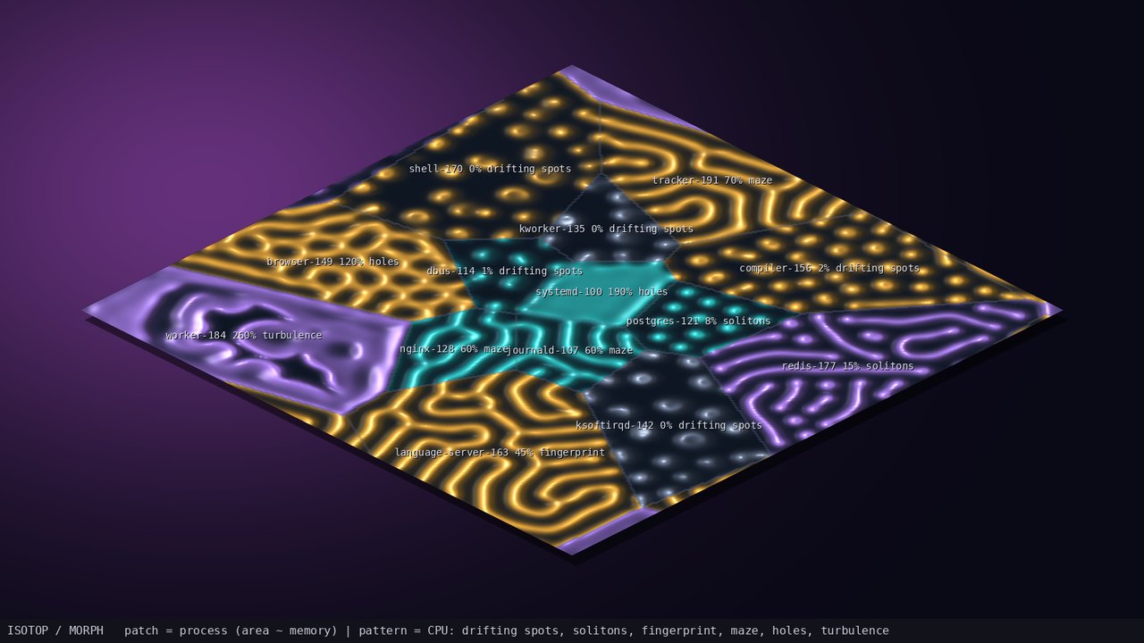
The reference still, docs/mockups/morph.jpg, rendered by the Python prototype docs/mockups/code/morph.py from synthetic data. It is a visual target, not a render of isotop.

1. The system being modelled

Morphogenesis is the problem of how a featureless embryo gets a spatial pattern. Turing's 1952 answer was that two reacting, diffusing chemicals can destabilise a uniform state and leave a standing pattern with a wavelength set by chemistry alone; the Gray-Scott model is a two-line chemical system in which that family of patterns, and some that Turing's linear argument does not reach, can be explored by turning two knobs, a feed rate $F$ and a kill rate $k$.

It is a good metaphor for process data for one reason that is almost mechanical: the knobs are a continuous driving of a dissipative system, and the morphology is a classification of the driving. A process that does nothing leaves the medium barely fed and the pattern sparse; a process that burns many cores drives the medium into regimes where fronts keep splitting and merging. CPU is a natural driver. It is also an honest limit: the metaphor says "more CPU means a busier-looking pattern", not "this pattern means this CPU" (see section 5).

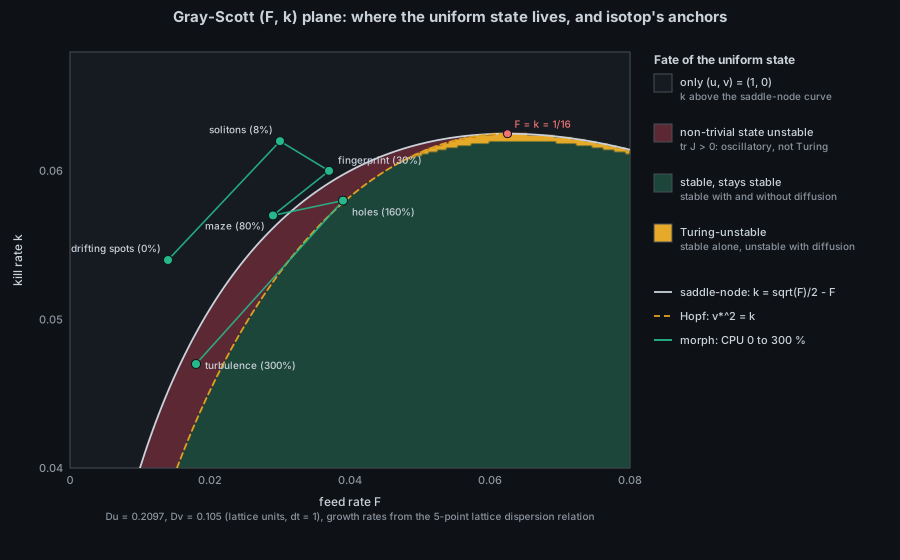
The theory (fixed points, the saddle-node and Hopf curves, the Turing condition, the finding that none of the six isotop anchors is a classical Turing pattern) is derived in Math-Reaction-Diffusion. The short version needed here:

$$ \partial_t u = D_u \nabla^2 u - u v^2 + F(1-u), \qquad \partial_t v = D_v \nabla^2 v + u v^2 - (F+k),v , $$

the trivial state $(u,v) = (1,0)$ is always stable, so patterns need finite-amplitude seeds, and a patch whose $v$ has vanished cannot revive itself.

History

The question is older than chemistry's answer to it. How a uniform egg becomes a patterned animal was a standing problem of embryology when Alan Turing, in "The chemical basis of morphogenesis" (Philosophical Transactions of the Royal Society B 237, 1952, pp. 37-72), showed that two reacting and diffusing substances can destabilise a uniform state and leave a stationary pattern whose scale is set by the chemistry. It was one of the last papers he published; he died in 1954. For some decades the idea was admired and not demonstrated.

The chemistry came from engineers. P. Gray and S. K. Scott studied the autocatalytic step $A + 2B \to 3B$ in a continuously stirred reactor in papers of 1983 and 1984 (Chemical Engineering Science 38 and 39); their model, with diffusion added, is the one on this page and is named after them. A Turing-type standing pattern was first made in the laboratory in 1990, in a gel fed with the chlorite-iodide-malonic acid reaction, by V. Castets, E. Dulos, J. Boissonade and P. De Kepper (Physical Review Letters 64, pp. 2953-2956). In the same 1993 issue of Science, K. J. Lee, W. D. McCormick, Q. Ouyang and H. L. Swinney reported patterns in a gel reactor, and John E. Pearson published "Complex patterns in a simple system" (Science 261, pp. 189-192), a numerical survey of the Gray-Scott equations, in which irregular patterns and spots that divide appear as the feed and kill rates are varied. The $(F,k)$ plane used by this view descends from that survey.

Whether animals do this is a separate, still argued matter. S. Kondo and R. Asai reported in 1995 (Nature 376, pp. 765-768) that the stripes of the marine angelfish Pomacanthus are not fixed once and for all: they drift as the fish grows, and a new stripe appears when the body reaches roughly 4 cm, which is what a reaction-diffusion wave would do.

The word in the page title has a second career. Image morphing, the warping and cross-dissolving of one picture into another from pairs of feature lines, was described by T. Beier and S. Neely in SIGGRAPH 1992 (Computer Graphics 26(2), pp. 35-42). The dish on this page never turns into anything but itself.

2. Theory specific to this design

2.1 From CPU to $(F, k)$

The brief fixes six anchors and interpolates linearly in $\log(1 + \text{cpu})$ between them, with CPU in percent of one core clamped to 300 %:

CPU %	$F$	$k$	Look
0	0.014	0.054	drifting spots
8	0.030	0.062	solitons
30	0.037	0.060	fingerprint
80	0.029	0.057	maze
160	0.039	0.058	holes
300	0.018	0.047	turbulence

The brief warns against the classic "chaos" preset $(0.026, 0.051)$ for the top end: in the prototype it settled into a flat, low-contrast fill. The interpolation, computed with the helper in docs/figures/rdsim_w8.py, gives for example:

CPU %	1	2	5	15	50	120	220
$F$	0.0190	0.0220	0.0270	0.0333	0.0329	0.0348	0.0284
$k$	0.0565	0.0580	0.0605	0.0611	0.0584	0.0576	0.0524

Because $F$ and $k$ are piecewise linear in $\log(1+\text{cpu})$, the path in the $(F,k)$ plane is a polyline through the anchors, drawn in the aqua line of the plane figure of Math-Reaction-Diffusion. The anchor positions relative to the saddle-node and Hopf curves show why the mapping is a heuristic and not a derived law: four of the six anchors lie where no non-trivial uniform state exists at all.

2.2 The dish, the stencil and the clock

• Grid. A fixed 256 x 256 dish with zero-flux (clamped) edges and no wrap, so every patch is one contiguous region. (The prototype wraps; the issue is explicit that this one does not.)
• Stencil. Sims's 9-point kernel (0.2 on edges, 0.05 on corners, $-1$ at the centre) with $D_u = 0.699$, $D_v = 0.35$, $\Delta t = 1$. The kernel's symbol along an axis is $-0.3 \cdot 2(1-\cos q)$, so this is the same continuum diffusion as $D_u = 0.2097$, $D_v = 0.105$ with the 5-point stencil, and explicit Euler is stable (the kernel's symbol reaches $-1.6$ at the corners of the Brillouin zone, so $D \le 1.25$ is allowed).
• Clock. simulation::FixedStep at 240 steps per second of view time, at most 48 steps per frame. Cost arithmetic: $256^2 \times 240 = 15.7$ million cell-updates per second. At 60 fps that is 4 steps per frame; at 5 fps it is exactly the cap of 48. Below 5 fps the dish runs in slow motion, because FixedStep drops the time it cannot catch up (it keeps accumulator.min(step)). Time that does not advance (pause, rewind) takes no steps.
• Settling. On creation the dish runs 1500 steps (6.25 s of view time) so that the first frame is already patterned, live and under --output. In the stdlib prototype of Math-Reaction-Diffusion, 10000 steps were needed before the anchors looked settled on a small dish, so a first frame will show a young pattern (not measured for the 256 x 256 dish; see section 8).

2.3 Patches: a power diagram

Patch borders are a power diagram (a weighted Voronoi diagram): a cell belongs to the process minimising $\lvert x - s_i\rvert^2 - w_i$, where $s_i$ is the process's site and

$$ w_i = 0.01 \cdot \frac{256^2}{n} \cdot \ln(1 + \text{MiB}_i), $$

with $\ln(1+\text{MiB})$ quantised to steps of 0.25. For 14 processes on 300 cells this reproduces the prototype's $60\ln(1+\text{MiB})$. Each process also always owns at least its site cell.

Sites come from the lifetime seat of the process (the issue calls the helper pack::Seats; in the tree the same thing is layout::Seats in src/layout.rs): seat $s$ is the point

$$ \bigl(\operatorname{frac}(0.5 + 0.7548777,s),\ \operatorname{frac}(0.5 + 0.5698403,s)\bigr) $$

scaled into the dish and inset 4 cells from the edge, never moved. The two constants are $1/\rho$ and $1/\rho^2$ where $\rho = 1.3247\ldots$ is the plastic number (the real root of $x^3 = x + 1$): the R2 sequence, a two-dimensional low-discrepancy sequence (popularised by M. Roberts in 2018, a web article), the plane's analogue of the golden-ratio rotation. Consecutive seats are spread out, so a newcomer never lands on top of an existing site.

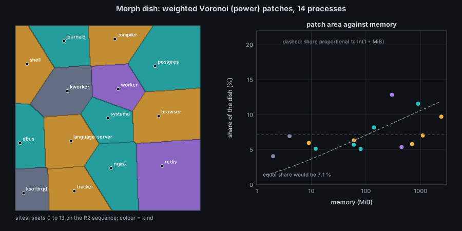
docs/figures/morph-power-diagram.py: the prototype's 14 processes on R2 sites with the issue's weights (my reading of the inset as $4 + \text{frac}\times 248$, and of the rounding, is an assumption).

A computed caution about "area ~ memory". With these weights the memory effect is small. With all weights zero (a plain Voronoi diagram on the same R2 sites) the 14 shares already range from 4.2 % to 12.9 %. Switching on the issue's weights changes no process's share by more than 0.49 percentage points. The rank correlation between memory and share is 0.52 without weights and 0.55 with them; scaling the weights five-fold raises it to 0.76. The reason is dimensional: $w$ is at most $0.01,(A/n) \ln(1+\text{MiB})$, about $0.08,(A/n)$ for a multi-GiB process, while the site spacing squared is of order $A/n$, so a border shifts by only a few per cent of the spacing. So at the specified constants patch size is dominated by where the seat falls, not by memory; the legend's "area ~ memory" is, as specified, a weak statement. This is a finding about the specified design, not an observation of isotop code.

2.4 Lifecycle rules

• Birth. Seed $v$ with 8 nuclei drawn from simulation::Rng::for_identity(id, salt) in the new patch.
• Reseed. On each sample a live patch with $\max v < 0.05$ gets 3 nuclei. This is physically necessary: see the stability of the trivial state in Math-Reaction-Diffusion.
• Exit. The patch keeps its owner as a ghost with $F = 0$, $k = 0.06$. The ghost ends when $\max v < 0.01$ or after 1920 steps (8 s), whichever is first; its cells then go to its neighbours and its seat is freed. The timeout is counted in simulation steps, never wall clock, so renders repeat. Ghost cells are unpickable.
• Zombie (Z) and stopped (T) patches skip updates (neighbours still read their cells). D state desaturates the patch by 60 %.

An isolated periodic test patch shows that starvation is fast: switching a settled pattern to $F = 0$, $k = 0.06$ takes $\max v$ below 0.01 in under 100 steps (0.4 s at 240 steps/s) for every anchor state tried. The 1920-step timeout is therefore a safety limit, and visible starvation will usually be over in well under a second; a border patch coupled to live neighbours can take longer. The brief's "starves within seconds" is, on this test, conservative.

3. Mapping

The realness contract: every visual element maps to a measured quantity or is declared decorative.

Visual element	Measured quantity (source)	Transform
Patch area	Process.memory (RSS; footprint on macOS)	power-diagram weight $0.01(256^2/n)\ln(1+\text{MiB})$, $\ln$ quantised to 0.25; owners recomputed on each sample or population change
Patch site	process identity (lifetime seat)	R2 point, inset 4 cells; never moves (Theory-Stable-Layout)
Pattern morphology	Process.cpu, percent of one core (EMA of $\Delta$ticks, $\tau = 1.5$ s, model::measure)	$(F,k)$ by anchor interpolation on $\log(1+\text{cpu})$, clamp 300 %, Gaussian blur $\sigma \approx 1.5$ cells across borders
Relief height	$v$ of the simulation	$0.6 \times \text{clamp}(v/0.33, 0, 1)$ world units
Tint	Process.kind via kind_color	height-shaded
Frozen patch	Process.state Z or T	no update
Desaturated patch	Process.state D (Linux only)	$-60,%$ saturation
Starving patch	process exit	$F=0$, $k=0.06$, then handed to neighbours
Faint borders	owner changes	drawn where the owner grid changes
Label text	name, CPU %, look name	look = nearest anchor on the log axis; no Greek letters
Pattern detail (where each spot sits)	none	seeded from Rng::for_identity; decorative
Dish slab sides and shadow	none	decorative

4. Design: how isotop will realise it

• Module. src/morph.rs, a #[derive(Default)] state struct implementing views::ViewModule, with the pure simulation state kept separate from drawing (as medium.rs does). One row at the end of views::REGISTRY, built with ViewInfo::new(name, title, backdrop, build): name morph, status name MORPH, Backdrop::Dusk, build a closure returning the boxed module, available left at its default (everywhere), no view-local key, no digit. Pure state in Morph; draw(&mut Stage, &[&Process], &Snapshot) -> usize.
• Data. Only existing fields: cpu, memory, state, kind, name, id. No new Process fields and no model::demo changes: the demo already spans 0 to about 320 % CPU and contains Z, T and D states.
• Rendering. The P3 field primitive in relief mode (a lit heightfield with an owner grid for picking), identical on the CPU and GPU rasterizers. Per-cell colours and heights are baked on the CPU. The slab sides and shadow are plain quads. Hovering a patch picks its process through the owner grid; ghost cells give NONE.
• Performance. $u$ and $v$ as f32 structure-of-arrays with a back buffer, the interior loop without bounds checks and the edges separately; if --processes 1000 misses 5 fps the rows are split over std::thread::scope (the Jacobi update keeps results bit-identical). Owners are recomputed only when a sample arrives or the population changes, pruned per 16 x 16 tile, target under 5 ms at 192 processes.
• Determinism. Per-process randomness is Rng::for_identity; the stepping is a pure function of the step count; two renders of the same --time are byte-identical (Theory-Determinism). Headless runs warm up the dish through the P1 registry row's warm-up declaration.
• Text. Labels for the 12 largest live patches read label_name cpu% class through stage.places; the inspector shows pattern: maze F 0.0290 k 0.0570, patch: N cells (x% of dish) and frozen (stopped). Legend: patch = process (area ~ memory) | pattern = CPU: spots, solitons, fingerprint, maze, holes, turbulence | frozen = stopped. All process text passes through the sanitizer (Theory-Text-Safety).
• Dependencies (ROADMAP index): P1 registry, P2 picker, P3 field primitive, S1 parity check, S2 simulation::FixedStep. In the current tree all five are merged, P3 included (Field, Relief and Frame::field in src/render/field.rs); nothing blocks the view except writing it.
• Platforms. Linux: available. macOS: available; every consumed field exists on both platforms. macOS never reports the D state, so desaturation does not occur there. There are no degraded sources and no missing-source text in the legend.
• No plugin system. Like every view, morph is a compile-time module and a REGISTRY row; nothing loads dynamically.

5. Reading the picture

• Measured: the patch's existence and border (the process, its memory through a weak weight), its tint (kind), whether it is frozen or desaturated, and a CPU-ordered morphology class.
• Derived: the pattern. It is the output of a simulation driven by smoothed CPU, so it carries memory: a patch's morphology reflects the CPU of roughly the last tens of seconds, not the last sample, because the pattern's relaxation time is thousands of steps (several seconds to tens of seconds of view time). A reaction-diffusion medium can also stay in a pattern when the parameters move a little (multistability, a standard property of this family; not yet observed in isotop).
• Decorative: where exactly spots and stripes fall; the slab and its shadow.
• Cannot infer: CPU from the pattern (the $(F,k)$ path doubles back in $F$ above 160 %); memory from patch area (section 2.3); anything about the order of events from the pattern's age.
• Resolution: a 256 x 256 dish shared by 192 processes gives about 340 cells per patch on average, a patch about 18 cells wide, only a bit more than one wavelength of the finer patterns. Small patches cannot show a maze (the brief's own test uses 128 x 128 for one process). Expect small patches to read as spots whatever their CPU.

6. Try it

Nothing runs in isotop yet. When the view lands the commands will be:

./target/release/isotop --demo --view morph --time 12 --width 1600 --output /tmp/morph.png --renderer cpu

(--view morph, Tab and the v picker will reach it; no digit.) Today you can regenerate the page's figures and explore the model:

python3 docs/figures/morph-power-diagram.py
python3 docs/figures/reaction-diffusion-patterns.py

7. Where in the code

Existing infrastructure the design will use: simulation::FixedStep, simulation::Rng::for_identity, simulation::smoothstep and smoothing in src/simulation.rs; layout::Seats in src/layout.rs; palette::kind_color in src/palette.rs; render::label_name and Stage in src/render.rs; terminal::clean_text in src/terminal.rs; views::ViewInfo, views::ViewModule and REGISTRY in src/views.rs; the field primitive (Field, Relief, Frame::field) in src/render/field.rs; the CPU smoothing in model::measure in src/model.rs (smoothing(dt, 1.5)). Planned: src/morph.rs; the R2 helper the issue puts in pack.rs (there is no pack.rs; layout.rs is its home); the prototype docs/mockups/code/morph.py (numpy and scipy, reference only).

8. Variations and open questions

• Make memory visible: raise the weight scale (the computed rank correlation reaches 0.76 at five times the issue's constant) or make area proportional by iterating weights to a target area (a capacity-constrained power diagram).
• Measure how many of the 1500 settle steps a 256 x 256 dish needs before the six morphologies are recognisable, and whether a warm start from a stored settled field would be better.
• Test hysteresis: ramp a patch's CPU up and down and look for different morphologies at the same CPU.
• Replace the log-linear anchor interpolation by a path through a measured Pearson map that avoids dead zones.
• Add a pressure-driven global bias (a uniform $k$ shift) so the whole dish "feels" memory pressure.

9. References

• A. M. Turing, "The chemical basis of morphogenesis", Philosophical Transactions of the Royal Society B 237 (1952).
• P. Gray and S. K. Scott, Chemical Engineering Science 38 (1983) and 39 (1984), on the autocatalytic reaction $A + 2B \to 3B$.
• J. E. Pearson, "Complex patterns in a simple system", Science 261 (1993) 189-192.
• K. Sims, "Reaction-Diffusion Tutorial" (web page); R. Munafo, "xmorphia" (web pages).
• M. Roberts, "The Unreasonable Effectiveness of Quasirandom Sequences" (web article, 2018), for the R2 sequence.
• Issue #50; docs/briefs/views-2026-10.md section 11; docs/VIEW_CONVENTIONS.md.