Math Wave Equation

Math: the wave equation on a lattice

The Ripple view is a pond: a two-dimensional membrane, a grid of heights and velocities, kicked by the processes that run on the machine. This page is the mathematics under it, independent of any one view: where the wave equation comes from, what a finite-difference scheme does to it, why there is a speed limit on the time step, how much the lattice distorts the waves, and how a boundary that is only a grid edge can be made to swallow them. Every parameter quoted for isotop is read from src/medium.rs; the view that uses the scheme is View Ripple.

The page keeps three things apart. Theory is standard numerical analysis and physics and would be the same in any program. Code is what Wave in medium.rs does. Inference is what the pictures let you conclude. Numbers marked measured come from a stdlib Python port of Wave::step and Wave::advance that reproduces the Rust unit test waves_spread_at_their_speed_and_die_out_at_the_border (a ring at $ct$ against none at $2ct$, and an energy fall of about $2\times10^{-7}$ over 30 s); they are not read off the binary.

History

The equation was first written for a violin string. Jean le Rond d'Alembert derived the one-dimensional wave equation in 1747 and found its general solution as the sum of two shapes travelling in opposite directions. Euler took it up in 1748 and 1749 and showed how to build the solution from the initial shape. Daniel Bernoulli countered that any motion of the string is an infinite sum of sine harmonics, without being able to say how to find the coefficients. The three disagreed for decades over a question that sounds modest: whether an initial shape with a corner, such as a plucked string, counts as a function at all. D'Alembert and Euler wanted a single analytic expression; Bernoulli argued on physical grounds that the plucked string existed whether or not the mathematics approved.

Fourier's work on heat (presented 1807, published in book form in 1822) supplied the missing coefficient formula, and Dirichlet's 1829 convergence theorem is the usual date given for the end of the argument. The two-dimensional membrane and the three-dimensional wave followed in the 19th century; Hadamard's Lectures on Cauchy's Problem (1923) gave the reason that sharp signals leave no tail in three dimensions but do in two, the fact the Huygens section above relies on.

The lattice came later and from a different motive. Courant, Friedrichs and Lewy published their paper in Mathematische Annalen in 1928 to prove that solutions of such equations exist, by showing that finite-difference approximations converge. The condition on the time step that every explicit wave solver since has had to respect appeared there as a by-product, and the machines it would constrain did not yet exist. The sponge at the border descends from the 1970s and 1980s work on artificial boundaries (Engquist and Majda 1977; Israeli and Orszag 1981); Berenger's perfectly matched layer followed in 1994.

The equation

A membrane of surface density $\sigma$ under isotropic tension $T$, displaced by $h(x,y,t)$ a little from flat, has the transverse force on a patch $T,\nabla^2 h,\mathrm{d}A$ (the net pull of the neighbouring sheet, linearised for small slopes) and mass $\sigma,\mathrm{d}A$. Newton's second law gives

$$ h_{tt} = c^2 \nabla^2 h, \qquad c^2 = T/\sigma . $$

In one dimension this is d'Alembert's equation, $h = f(x - ct) + g(x + ct)$: shapes travel unchanged. In two dimensions a plane wave $e^{i(\mathbf{k}\cdot\mathbf{x} - \omega t)}$ solves it when $\omega = c\lvert\mathbf{k}\rvert$: every wavelength travels at the same speed, so the medium is non-dispersive.

Real water is not this medium. Surface waves on a pond obey $\omega^2 = (gk + \tau k^3/\rho)\tanh(kd)$ with gravity, surface tension and depth, which is dispersive and has no single speed (Lamb 1932). The pond in isotop is a membrane analogy: the tidy equation, chosen because it is cheap, linear, and gives interference you can see.

What isotop actually integrates

Wave in medium.rs integrates a damped Klein-Gordon equation with a forcing term:

$$ h_{tt} = c^2 \nabla^2 h ;-; \gamma(\mathbf{x}), h_t ;-; \kappa, h ;+; F(\mathbf{x}, t), $$

with $c = 14$ cells per second (WAVE_SPEED), a background $\gamma = 0.35\ \mathrm{s^{-1}}$ (DAMPING) raised near the border by a sponge (below), $\kappa = 0.5\ \mathrm{s^{-2}}$ (RESTORE), and $F$ the pebbles' forcing. The comment in the source gives the reason for $\kappa$: a uniform offset has no curvature, so without a pull back to rest the impulses of births and exits would leave the whole pond permanently raised or lowered. Space is measured in grid cells: the code never divides by the cell size, so $c$ is 14 cells per second whatever the world-space size of the cell is (see the view page for what that does to the picture).

Dispersion of the continuum equation

Put $h = e^{i(kx - \omega t)}$ in the homogeneous equation:

$$ \omega^2 + i\gamma\omega = c^2 k^2 + \kappa . $$

Three consequences, each used later.

1. Cutoff. With $\gamma = 0$, $\omega^2 = c^2k^2 + \kappa$: waves exist only above $\omega_c = \sqrt{\kappa} = 0.707\ \mathrm{rad/s}$ (0.113 Hz). The pebbles sound at 0.35 to 1.25 Hz, well above it.
2. Mild dispersion. Phase speed $v_\varphi = c,\omega/\sqrt{\omega^2-\kappa}$ and group speed $v_g = c\sqrt{\omega^2-\kappa}/\omega$. At 0.35 Hz these are $1.056,c$ and $0.947,c$; at 1.25 Hz, $1.004,c$ and $0.996,c$. The restoring term makes long waves slightly dispersive, and that is a larger departure than the lattice causes at the same end of the band.
3. Spatial decay of a driven wave. At real driving frequency the wavenumber is complex, $k^2 = (\omega^2 - \kappa + i\gamma\omega)/c^2$, and for $\gamma \ll \omega$

$$ \operatorname{Im} k ;\approx; \frac{\gamma,\omega}{2c\sqrt{\omega^2-\kappa}} ;\approx; \frac{\gamma}{2c} . $$

With $\gamma = 0.35$ and $c = 14$ this is 0.0126 per cell (amplitude e-folding over 79 cells). Measured: a point source at 0.8 Hz on a $301\times201$ grid gives an envelope falling as $r^{-1/2}e^{-\alpha r}$ with $\alpha = 0.0122$ between 10 and 40 cells, within 4% of the formula.

Why a point source leaves a wake: Huygens in two dimensions

The response of the undamped two-dimensional equation to an initial velocity impulse $h_t(\mathbf{x},0) = \delta(\mathbf{x})$ is

$$ G(r,t) = \frac{1}{2\pi c},\frac{\Theta(ct - r)}{\sqrt{c^2t^2 - r^2}}, $$

with $\Theta$ the unit step. There is a sharp front at $r = ct$, but behind it the disturbance does not return to zero: it decays as $1/(ct)$ and persists. In three dimensions the Green's function is supported on the sphere $r = ct$ alone (Huygens' principle in the strict sense: sharp signals, no tail); in even dimensions it has a tail (Hadamard, Lectures on Cauchy's Problem, 1923; Courant and Hilbert vol. II). A drip on a two-dimensional membrane therefore leaves a mound that drains slowly, and the births and exits in isotop (impulses of $+30$ and $-90$ on the velocity, see below) show this: the $\kappa$ term and the damping are what finally return the pond to rest. Fresnel's and Huygens' picture of every point of a wavefront as a secondary source remains a good construction, but in 2D the secondary wavelets must carry their tails.

The lattice

Cover the plane with a square grid of spacing $\Delta x$ (taken as 1; isotop's code does the same) and replace $\nabla^2$ by a stencil.

Five and nine points

The five-point Laplacian $L_5 h = h_{E}+h_{W}+h_{N}+h_{S} - 4h$ has symbol (the factor it multiplies a plane wave by) $-s_5(\mathbf{k})$ with

$$ s_5 = 4 - 2\cos k_x - 2\cos k_y = k^2 - \tfrac{1}{12}\left(k_x^4 + k_y^4\right) + O(k^6). $$

The leading error depends on direction: it is $k^4/12$ along an axis and $k^4/24$ along a diagonal. A wave that should be round is slower along the axes than along the diagonals, and rings square off.

Wave::step uses the nine-point stencil

$$ \nabla^2 h \approx \frac{1}{6}\Big[,4,(h_E+h_W+h_N+h_S) + (h_{NE}+h_{NW}+h_{SE}+h_{SW}) - 20,h,\Big], $$

which is a blend $\tfrac{2}{3}L_5 + \tfrac{1}{3}L_\times$ of the five-point stencil and the same stencil on the lattice rotated 45 degrees ($L_\times h = \tfrac12(\text{diagonals} - 4h)$). The diagonal stencil has symbol error $\tfrac{1}{12}(k_x^4+k_y^4) + \tfrac12 k_x^2k_y^2$, and the weights 2/3 and 1/3 are exactly those that cancel the direction-dependent part:

$$ s_9 = \frac{20 - 8\cos k_x - 8\cos k_y - 4\cos k_x\cos k_y}{6} = k^2 - \frac{1}{12},k^4 + O(k^6). $$

The $k^4$ term is a function of $\lvert\mathbf{k}\rvert$ only: the stencil is $\nabla^2 h + \tfrac{\Delta x^2}{12}\nabla^4 h + O(\Delta x^4)$, second-order accurate and isotropic through the leading error. The directional spread appears only at $O(k^6)$. The comment in medium.rs ("its error is nearly isotropic, so rings stay round instead of squaring off along the grid axes") is exactly this. I checked the expansions numerically: at $k=0.1$ the fitted $(s - k^2)/k^4$ is $-0.0833$ for the nine-point stencil at 0, 0.3 and 45 degrees, and $-(\cos^4\theta+\sin^4\theta)/12$ for five points.

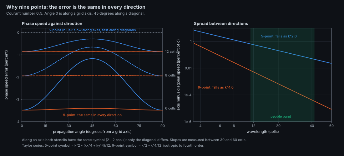
The measured spread between axis and diagonal falls as $k^{2.0}$ for five points and $k^{4.0}$ for nine. At the shortest pebble wavelength (11 cells) the five-point stencil would differ by 0.65% between axis and diagonal (at Courant number 0.5); the nine-point stencil by 0.007%.

The cost of the lattice: numerical dispersion

Put a plane wave in the semi-discrete system: $\omega_s = c\sqrt{s(\mathbf{k})}$. Along an axis $s = 2 - 2\cos k = 4\sin^2(k/2)$, so $\omega_s = 2c\sin(k/2)$ and the phase speed is $c,\sin(k/2)/(k/2) \approx c,(1 - k^2/24)$. Short waves lag, long ones do not: numerical dispersion, shown in the left panels below (the two stencils coincide along an axis).

Time stepping

Wave::step updates, for each interior node,

$$ v \leftarrow v + \Delta t,\big(c^2 \nabla^2 h - \gamma v - \kappa h\big), \qquad h \leftarrow h + \Delta t, v , $$

with the new $v$ in the second line: semi-implicit (symplectic) Euler, the kick-drift form of leapfrog. With $\gamma = 0$, eliminating $v$ (use $h^n = h^{n-1} + \Delta t,v^n$) gives

$$ \frac{h^{n+1} - 2h^n + h^{n-1}}{\Delta t^2} = c^2\nabla^2 h^n - \kappa h^n, $$

the classical second-order central scheme; the stored $v$ is the half-step velocity $v^{n+1/2}$. For a Hamiltonian system a symplectic step conserves a nearby modified energy rather than drifting (Hairer, Lubich and Wanner), so with the damping and the sponge switched off the pond neither gains nor loses energy secularly; all of its decay is the $\gamma$ term. For a plane wave

$$ \sin!\Big(\frac{\omega,\Delta t}{2}\Big) = \frac{\Delta t}{2}\sqrt{c^2 s(\mathbf{k}) + \kappa}, $$

so time stepping adds $+\nu^2k^2/24$ to the relative phase speed, with the Courant number $\nu = c,\Delta t/\Delta x$, against the lattice's $-k^2/24$:

$$ \frac{v_\varphi}{c} - 1 ;\approx; -\frac{(1-\nu^2),k^2}{24}, \qquad \frac{v_g}{c} - 1 ;\approx; -\frac{(1-\nu^2),k^2}{8}. $$

For $\nu = 0.5$ (isotop's largest) and the shortest pebble wavelength $\lambda = 11.25$ cells ($k = 0.559$): $-0.98%$ in phase speed, measured $-0.99%$ along an axis and $-0.98%$ along a diagonal; and $-2.9%$ in group speed. A wave packet crossing the 150-cell pond (10.7 s) at that wavelength arrives about three cells, a quarter wavelength, late.

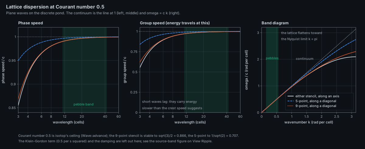
The band diagram (right) shows what the pebbles use: their $k$ runs from 0.149 to 0.559 radians per cell, the first fifth of the Brillouin zone $[0,\pi]$, where the lattice is almost linear. Nothing in the Ripple view lives near the Nyquist limit $k=\pi$ (wavelength two cells), where the group speed goes to zero along an axis and the scheme's behaviour is purely numerical.

Stability: the speed limit

Take one Fourier mode. Let $a = c^2 s(\mathbf{k}) + \kappa$. The update acts on $(h, v)$ by

$$ M = \begin{pmatrix} 1 - a\Delta t^2 & \Delta t,(1-\gamma\Delta t) \ -a\Delta t & 1 - \gamma\Delta t \end{pmatrix}, \qquad \operatorname{tr} M = 2 - a\Delta t^2 - \gamma\Delta t, \quad \det M = 1 - \gamma\Delta t . $$

Both eigenvalues lie in the unit disc if and only if $\lvert\det M\rvert \le 1$ and $\lvert\operatorname{tr}M\rvert \le 1 + \det M$, which for non-negative $a$ reduces to

$$ a,\Delta t^2 ;\le; 4 - 2\gamma\Delta t, \qquad \gamma\Delta t \le 2 . $$

The worst mode is the highest-frequency one, $s_{\max}$. For the nine-point stencil that is $\mathbf{k} = (\pi,\pi)$: $s_9 = (20+8+8-4)/6 = 16/3$. For five points it is 8. With $\gamma = \kappa = 0$:

$$ \nu_{\max}^{(9)} = \frac{2}{\sqrt{16/3}} = \frac{\sqrt3}{2} = 0.866, \qquad \nu_{\max}^{(5)} = \frac{2}{\sqrt 8} = \frac{1}{\sqrt2} = 0.707 . $$

I confirmed this by computing the spectral radius of $M$ over a $60\times60$ lattice of modes: it is $1.000000$ at $\nu = 0.86$ and $1.0266$ at $0.8661$ for nine points, and for five points $1.000$ at $0.7071$ against $1.464$ at $0.72$. This is the von Neumann analysis; it agrees with, and is stricter than, the necessary condition of Courant, Friedrichs and Lewy (1928) that the numerical domain of dependence contain the physical one ($\nu \le 1$ for the nine-point footprint).

Damping lowers the limit: at the sponge's maximum $\gamma = 6.35$ and $\Delta t = 0.0357$ s, $\gamma\Delta t = 0.227$ and the bound becomes $a\Delta t^2 \le 3.55$, $\nu \le 0.815$.

What isotop does. Wave::advance(time, force) clamps the elapsed time to $[0, 0.25]$ s and takes steps = ceil(elapsed * WAVE_SPEED / 0.5) equal substeps, so $\Delta t \le 0.5/c$: the Courant number never exceeds 0.5. At the default --fps 10 (elapsed 0.1 s) that is three substeps of 0.0333 s, $\nu = 0.467$; at 30 fps one step, $\nu = 0.467$ again. The margin to the damped limit is a factor 1.6 and to the undamped limit 1.7. The explicit damping term needs $\gamma\Delta t < 2$: worst case 0.227. The medium is f32; the margin is wide enough that rounding is not a stability concern (the unit test runs it for 30 s without growth).

Boundaries

What the frame does

step loops over 1..h-1 and 1..w-1: the outermost ring of nodes is never updated, and drive refuses to write within one cell of it. Those nodes stay at $h = 0$, $v = 0$: a Dirichlet boundary, which reflects with a sign change. Left alone, the pond would ring like a drum.

The sponge

Wave::new raises the damping near each edge. With $e$ the distance in cells from the nearest edge ($e = 0$ on the frame):

$$ \gamma(e) = 0.35 + 6,\max!\Big(0,\ \frac{10 - e}{10}\Big)^{2}\ \ \mathrm{s^{-1}} \qquad (\texttt{SPONGE} = 6,\ \texttt{SPONGE_CELLS} = 10). $$

This is a sponge layer in the sense of Israeli and Orszag (1981), not a perfectly matched layer (Berenger 1994) and not a one-way radiation condition (Engquist and Majda 1977): it removes energy by friction, and a friction gradient reflects. A wave that enters the sponge loses amplitude by about $\exp(-\tfrac12\int\gamma,\mathrm{d}t)$ one way; with $\int_0^{10}(0.35+6d^2),\mathrm{d}e/c = 1.68$ the round trip is $e^{-1.68} = 0.19$ in amplitude.

I measured the reflection coefficient with the exact scheme at normal incidence (one-dimensional run, which is exact for an axis-aligned plane wave because the nine-point stencil reduces to the three-point one when nothing varies in $y$; a wide Ricker pulse, with the reflection isolated by subtracting a run on a domain 600 cells longer):

frequency	wavelength	amplitude reflected	energy reflected
0.35 Hz	40 cells	0.46	21%
0.50 Hz	28 cells	0.31	10%
0.80 Hz	17.5 cells	0.18	3.2%
1.00 Hz	14 cells	0.18	3.3%
1.25 Hz	11.2 cells	0.19	3.4%

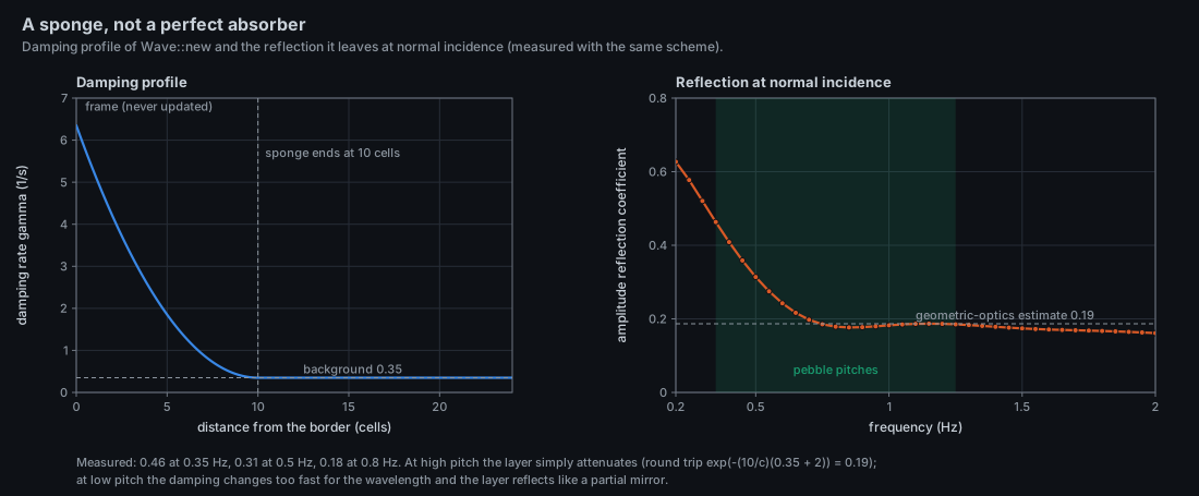
At the short-wavelength end the reflection is the geometric-optics estimate 0.19; at long wavelengths the damping changes too quickly relative to the wavelength and the layer reflects like a partial mirror, up to 46% in amplitude at the lowest pebble pitch. Oblique waves should reflect more, since the component of the wavelength across the layer is longer (expected, not measured). The border therefore absorbs, but is not an absorbing boundary condition in the strict sense, and the background $\gamma = 0.35$ does a good deal of the work: it alone reduces a ripple by $e^{-0.175,t}$, a factor 0.15 over a 10.7 s crossing.

Where the layout sits

cover (called by footprint in the Ripple view) pads the layout by margin = 8 + 0.08 * extent world units on each side and covers it with 150 cells on the longer side. With $L$ the layout's longer extent the margin in cells is $10.34,(L+100)/(L+13.8)$, which is at least 10.34 for every $L$ and 14.5 at $L = 200$. The sponge is 10 cells wide, so no pebble ever sits inside it, whatever the machine's size. (The margin rule is render::cover in render.rs and the 150-cell grid is the argument footprint in views/ripple.rs passes to it; the match with the sponge width is not stated in a comment, so I treat it as design intent supported by arithmetic, not as a documented invariant.)

Forcing

Wave::drive(p, amount) adds amount times a fixed footprint to the velocity around the node nearest $p$: weight 1 at the centre, $\tfrac12$ on the four edge neighbours, $\tfrac14$ on the four diagonals. The footprint is separable, $\tfrac12^{\lvert dx\rvert}\cdot\tfrac12^{\lvert dy\rvert}$ with total weight 4, and its transform is $(1+\cos k_x)(1+\cos k_y)$: a raised-cosine low-pass that is exactly zero at the checkerboard mode $(\pi,\pi)$ and 15% below its peak at $k = 0.56$, so no source can excite the grid-scale mode that the stencil handles worst.

A pebble drives the pond with a force

$$ F(t) = 900,\frac{u}{u+40},\sin(2\pi f t + \varphi)\quad (u = \text{its CPU in percent}), $$

applied each substep as drive(at, loudness * sin(...) * dt), so that the velocity increment is $F,\Delta t$ as it should be for an acceleration. Births add an impulse $+30$ and exits $-90$ to the velocity at the point. The frequency $f$ and phase $\varphi$ come from a hash of the pid (see View Ripple); the theory does not care.

The steady response of the continuum equation to a point force of frequency $\omega$ is a Hankel wave, $h(r) \propto H_0^{(2)}(k r)$ with complex $k$, whose far field decays as $(k r)^{-1/2}e^{-\operatorname{Im}k, r}$. In two dimensions energy spreads over a circumference proportional to $r$, hence the $r^{-1/2}$ amplitude; the visible rings of a pebble are the near field of this Hankel function seen through the damping.

Exact parameters

symbol	name in medium.rs	value
$c$	WAVE_SPEED	14 cells per second
$\gamma_0$	DAMPING	0.35 per second
sponge strength	SPONGE	6 per second, quadratic in depth
sponge width	SPONGE_CELLS	10 cells
$\kappa$	RESTORE	0.5 per second squared
frame step clamp	in advance	elapsed in $[0, 0.25]$ s
substeps	in advance	$\lceil 28,\text{elapsed} \rceil$, so $\nu \le 0.5$
grid	Grid::covering(..., 150)	150 cells on the longer side (footprint in views/ripple.rs, through render::cover)
forcing footprint	Wave::drive	$[\tfrac12,1,\tfrac12]^{\otimes 2}$
scheme	Wave::step	nine-point Laplacian, symplectic Euler

What the pictures let you infer

• Wavelength and speed are real, the metric is not. In grid units everything above is exact for the scheme. World-space speed is $14\times$ the cell size, and the cell size changes with the layout (150 cells always span the layout plus margin), so the pond crosses in 10.7 s whatever the machine looks like. Compare wavelengths in cells, never in the world units the camera uses.
• A ripple's reach is set by the damping, not by the process. Amplitude falls by $e^{-1}$ in 79 cells at the pebble frequencies (before geometric spreading), independent of CPU. A louder process is a larger amplitude, not a longer range, until the amplitude falls under what the shading can show.
• Short waves arrive late. A packet at the shortest pitch lags by about 3% over the crossing, a quarter wavelength. It matters for the phase relationship between distant sources and is invisible in the shading otherwise.
• The edge reflects some. At low pitches the sponge sends back 20% to 46% of the amplitude at normal incidence, so a faint standing pattern near the border is expected, not a bug.
• Interference is exact superposition. The medium is linear, so any pattern is the sum of the single-source patterns; the marbled look of a busy pond is the sum of 130 or so Hankel waves of different pitch (in the demo at --time 12, about 130 of 192 processes exceed the 0.3% threshold), not a nonlinear effect.

Where in the code

• src/medium.rs: Wave (new, drive, step, advance, test-only energy), Grid::covering, the constants WAVE_SPEED, DAMPING, SPONGE, SPONGE_CELLS, RESTORE; test waves_spread_at_their_speed_and_die_out_at_the_border.
• src/views/ripple.rs: the ViewModule implementation of Ripple (sources, wave.advance) and footprint (the grid over the pebbles).
• src/render.rs: cover (grid and margin), similar (when the medium survives a layout change).
• Figure scripts: docs/figures/wave-dispersion.py, docs/figures/wave-anisotropy.py, docs/figures/wave-sponge-reflection.py (shared drawing helper docs/figures/figkit_w4.py).

Variations and open questions

• A perfectly matched layer. Replace the sponge by a split-field PML (Berenger) of the same 10 cells: the reflection should fall below 1% at all pitches and angles. The cost is auxiliary fields on the border ring only.
• A fourth-order stencil. The $k^4/12$ error of the nine-point Laplacian can be cancelled by the compact (Mehrstellen) correction on the right-hand side; that removes the $-k^2/24$ spatial error and leaves the time-stepping term $+\nu^2k^2/24$, so at 11 cells the phase error would go from $-0.98%$ to $+0.33%$ (arithmetic, not an experiment). Would anyone see it?
• Real water. Swap the $c^2k^2 + \kappa$ dispersion for capillary-gravity waves by adding a $\nabla^4$ term (a bending stiffness): short waves then run faster, the opposite of the lattice's lag, and the two could be tuned to cancel at one pitch.
• Anisotropy on purpose. A sheet with $c_x \ne c_y$ would make the pond an anisotropic medium; the pebbles' rings become ellipses, and the stencil weights would have to follow.
• Measure the wake. The 2D Green's function predicts a positive tail behind a drip; compare the lattice response at a probe with $1/\sqrt{c^2t^2-r^2}$, with and without $\kappa$, to see $\kappa$ turn the tail into ringing at $\omega_c$.
• Kappa as a mass. The restoring term makes the pond a Klein-Gordon field with angular cutoff $\omega_c = \sqrt{\kappa} = 0.707$ rad/s; at $c = 14$ cells per second its reduced Compton wavelength, $c/\omega_c$, is 19.8 cells. The pond is, in this sense, a universe whose lightest particle is about 13 percent of its width.
• Open: is the sponge's quadratic profile a good one for the 3 to 1 span of wavelengths here? A cubic or a cosine taper has lower reflection at long wavelengths for the same total damping.

References

• R. Courant, K. Friedrichs, H. Lewy, "Über die partiellen Differenzengleichungen der mathematischen Physik", Mathematische Annalen 100 (1928), 32-74.
• J. Hadamard, Lectures on Cauchy's Problem in Linear Partial Differential Equations (Yale University Press, 1923).
• R. Courant and D. Hilbert, Methods of Mathematical Physics, vol. II (Interscience, 1962).
• E. Hairer, C. Lubich, G. Wanner, Geometric Numerical Integration, 2nd ed. (Springer, 2006).
• J. W. Strikwerda, Finite Difference Schemes and Partial Differential Equations, 2nd ed. (SIAM, 2004).
• L. N. Trefethen, "Group velocity in finite difference schemes", SIAM Review 24 (1982), 113-136.
• R. Vichnevetsky and J. B. Bowles, Fourier Analysis of Numerical Approximations of Hyperbolic Equations (SIAM, 1982).
• M. Israeli and S. A. Orszag, "Approximation of radiation boundary conditions", Journal of Computational Physics 41 (1981), 115-135.
• B. Engquist and A. Majda, "Absorbing boundary conditions for the numerical simulation of waves", Mathematics of Computation 31 (1977), 629-651.
• J.-P. Berenger, "A perfectly matched layer for the absorption of electromagnetic waves", Journal of Computational Physics 114 (1994), 185-200.
• H. Lamb, Hydrodynamics, 6th ed. (Cambridge University Press, 1932).
• M. Patra and M. Karttunen, "Stencils with isotropic discretization error for differential operators", Numerical Methods for Partial Differential Equations 22 (2006), 936-953 (unverified page range).