View HR

View HR

A planetarium sky of processes in blackbody colours, with a key that sends every star flying to its place on a Hertzsprung-Russell diagram of the machine. In sky mode an idle process glows orange and a busy one white or blue-white; size and brightness follow memory on the astronomical magnitude scale; twinkle follows how erratic a process's CPU has been; every cgroup is a constellation, with stick figures drawn along its socket links; kernel threads, which hold no memory and so have no luminosity, are the dust of a Milky Way band. In diagram mode (m) the same stars are plotted with temperature (from CPU) increasing to the left and magnitude (from memory) running down the page, the machine's own main sequence is fitted through them, and every star is classified against it: K3 III for a mid-orange process far brighter than the machine's trend, DA for a hot, small one.

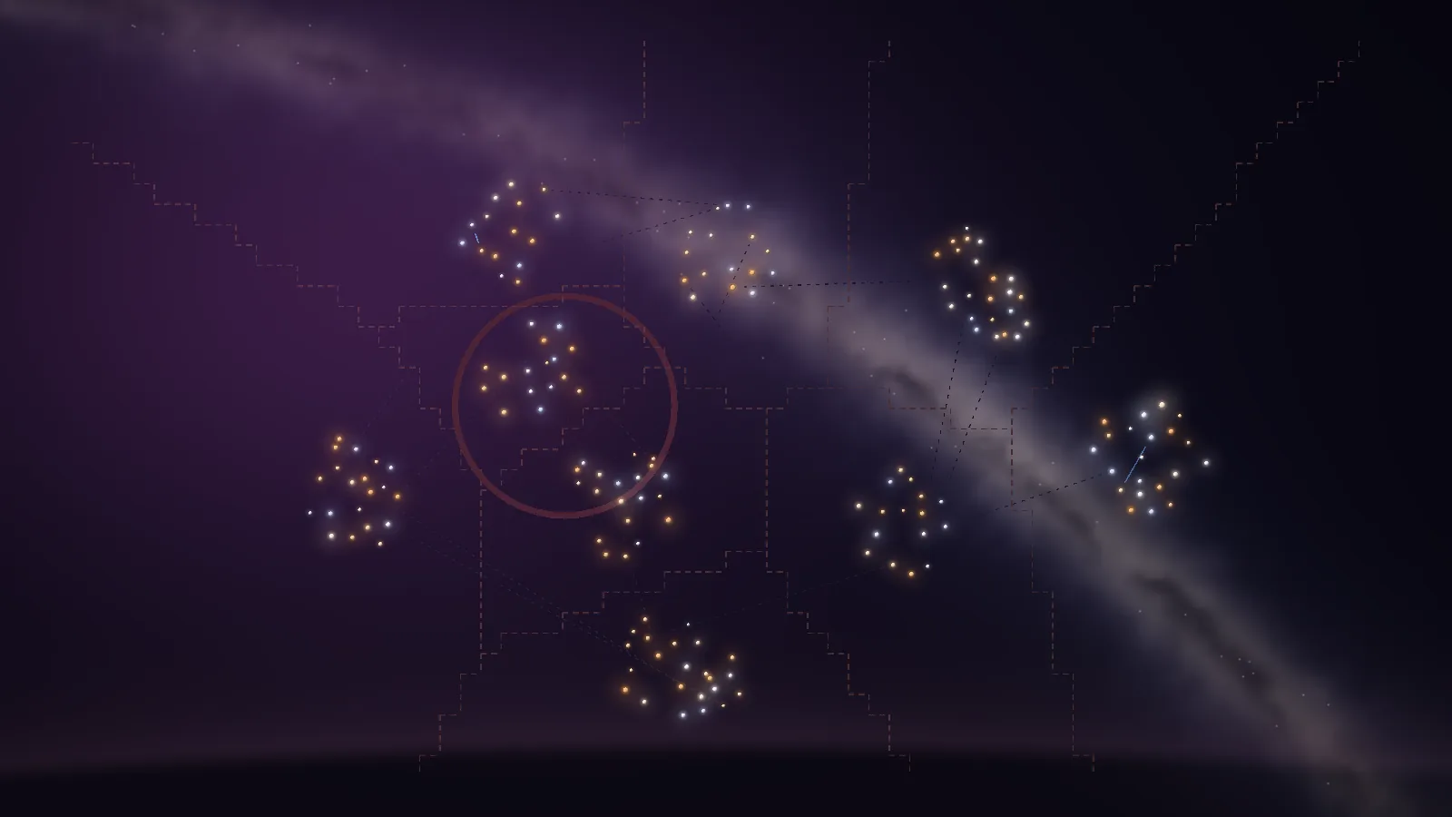
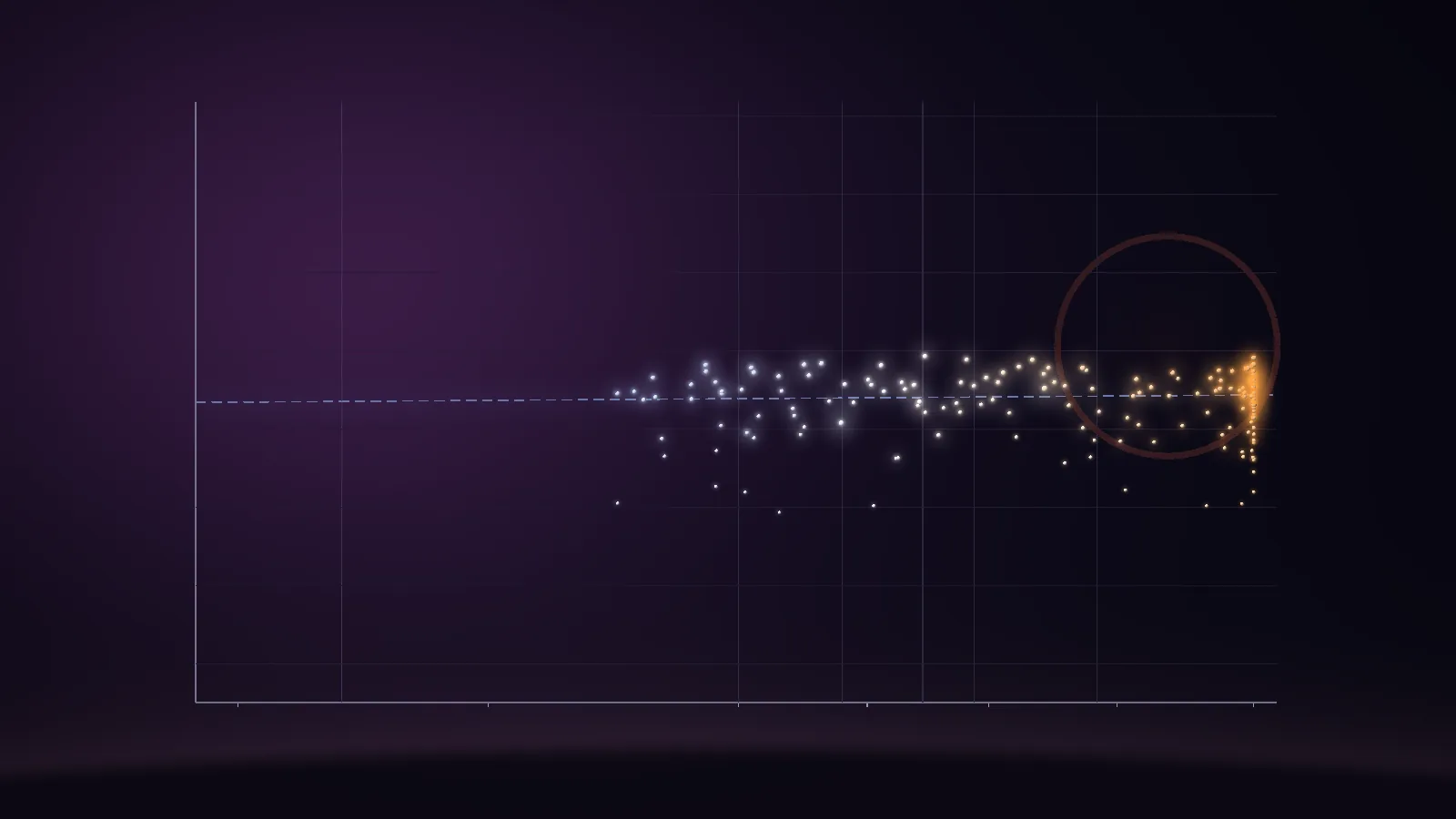
The demo workload at --time 12 (docs/media/hr.webp and docs/media/hr-diagram.webp, from --demo --view hr --time 12 --renderer cpu --width 1600, the second with --hr-diagram). Labels, constellation names and axis text are terminal text laid over the image, so they are not in the PNG. The ring is the shell of a supernova: a demo process of more than 1 GiB exited a few seconds earlier.

The system being modelled

The diagram. Around 1905 to 1911 Ejnar Hertzsprung noticed that among stars of the same colour some are far more luminous than others, and plotted the stars of the Pleiades and Hyades, which lie at a common distance, as colour against apparent magnitude. In 1913 Henry Norris Russell plotted spectral type against absolute magnitude for stars with measured parallaxes. The diagram that carries both names puts surface temperature (or colour, or spectral class) on the horizontal axis, with the hot end on the left by astronomers' convention, and luminosity on the vertical axis. Stars do not fill it: about nine in ten lie on a diagonal band, the main sequence, from hot and luminous (upper left) to cool and faint (lower right); the giants and supergiants sit above it on the right, cool but luminous; the white dwarfs sit far below on the left, hot but faint. The structure is physics, not a classification choice: the main sequence is where stars fuse hydrogen in the core, and a star's place on it is set by its mass; giants and white dwarfs are later stages.

Why the diagram is organised by temperature. The Stefan-Boltzmann law makes a surface of area $4\pi R^2$ at temperature $T$ radiate $L = 4\pi R^2\sigma T^4$. In logarithmic axes a star of radius $R$ lies on $\log L = 4\log T + 2\log R + \mathrm{const}$, a line of slope 4, so position off the main sequence is a statement about radius: a cool, luminous star must be huge, and a hot, faint one tiny. The vertical axis is usually a bolometric magnitude, $M_\mathrm{bol} = M_\mathrm{bol,\odot} - 2.5\log_{10}(L/L_\odot)$ with $M_\mathrm{bol,\odot} = 4.74$; five magnitudes are a factor of exactly 100 in flux, one magnitude $100^{1/5} = 2.512$, and a smaller number is brighter.

The classes. The Harvard sequence of spectral classes, hot to cool, is O B A F G K M, a sequence of surface temperature; each class is split into subclasses 0 to 9, hottest first. The Morgan-Keenan (Yerkes) system adds luminosity classes: I (supergiants, Ia brighter than Ib), II, III (giants), IV (subgiants), V (main sequence), VI (subdwarfs) and D (white dwarfs). The Sun, at 5772 K, is G2 V. "K3 III" is a cool orange giant.

Why it fits process data. A machine has no stellar physics, but it has the same organisation in two measured quantities: a heavy-tailed spread of memory (the luminosity axis) and a heavy-tailed spread of CPU (the temperature axis), with at most a rough correlation between them. A process far above the machine's own trend (a huge process doing almost nothing) is a "giant", and a small, busy one is a "white dwarf". The view makes this a diagnosis: the machine has a main sequence of its own, fitted every sample, and the classification names departures from it. It is a metaphor with real statistics underneath. It does not claim that processes obey a mass-luminosity relation.

History

Counting stars. The scale on the vertical axis began as a ranking. Hipparchus (2nd century BCE) is generally believed to have sorted stars into brightness classes in a catalogue that is lost, so the attribution cannot be proved. Ptolemy's Almagest (about 150 CE) lists 1,022 stars in 48 constellations by class, first magnitude brightest and sixth the faintest visible to the naked eye; nothing in that scheme was logarithmic. Abd al-Rahman al-Sufi revised the magnitudes in his Book of Fixed Stars (964 CE). In the 19th century photometers showed that a first-magnitude star gives roughly a hundred times the light of a sixth (John Herschel is usually credited with the observation, in the 1830s or 1840s; dates unverified), and in 1856 Norman Pogson, later director of the Madras Observatory, proposed making the ratio exact: five magnitudes a factor of 100, one magnitude 2.512. His paper, on thirty-six minor planets, is in the references. The zero point drifted for a century (Polaris, then Vega, then a standard sequence); the bolometric scale used for luminosity was pinned in 2015 by an IAU resolution at a luminosity of $3.0128\times10^{28}$ W for $M_\mathrm{bol} = 0$.

The Harvard computers. The horizontal axis is the work of the staff of the Harvard College Observatory. Edward C. Pickering, director from 1877, hired women as computers, a staff the newspapers nicknamed "Pickering's harem", and in 1886 Anna Palmer Draper endowed the Henry Draper Memorial to pay for classifying photographed spectra, in memory of her husband. Williamina Fleming, a Scot who had come to Boston in 1878 and been hired by Pickering in 1881, classified the spectra for the 1890 Draper Catalogue of Stellar Spectra (10,351 stars) by the strength of the hydrogen lines, A strongest down through Q; she also found the Horsehead Nebula on a plate in 1888. Antonia Maury, Draper's niece, published a more careful scheme in 1897: twenty-two groups ordered, in effect, by temperature, each with a lowercase letter for how sharp the lines were. Pickering preferred the simple letters. In 1905 Hertzsprung noticed that Maury's narrow-lined "c" stars had almost no proper motion, so were distant and therefore intrinsically luminous: the first luminosity classification, found in the margin of a scheme that had been set aside. Annie Jump Cannon, who joined the observatory in 1896 and was by then nearly deaf, dropped most of the letters and rearranged the survivors into O B A F G K M (published in 1901), added the decimal subclasses, and classified the stars of the Henry Draper Catalogue (nine volumes, 1918 to 1924, 225,300 stars) largely by eye; the International Astronomical Union adopted her sequence in 1922. The mnemonic that spells it is attributed to Harvard students and is best known as "Oh, be a fine girl, kiss me". The staff also produced Henrietta Leavitt, who in 1912 found that the brighter Cepheid variables of the Small Magellanic Cloud have the longer periods, and with it the first rung of the distance ladder. Dava Sobel's The Glass Universe (2016) is the readable account of the whole group.

Why the sequence is a temperature sequence. Cannon's letters were an ordering that nobody could explain. In 1920 Meghnad Saha derived how the ionisation of an atom depends on temperature and pressure, and in 1925 Cecilia Payne, in what is counted as the first astronomy doctoral thesis at Radcliffe, applied it to the Harvard spectra and showed that the classes differ in temperature, not in composition. She also found hydrogen and helium overwhelmingly more abundant than anything else; Russell, who read the thesis, thought that impossible, and she wrote in it that the result was almost certainly not real. Russell reached the same conclusion from his own analysis in 1929 and published it. Otto Struve is quoted as calling the thesis the most brilliant ever written in astronomy (as widely repeated; unverified). Payne married Sergei Gaposchkin in 1934, and in 1956 became a full professor and chair of the astronomy department, the first woman to chair a department at Harvard. Her The Galactic Novae (1957) is the classification Math: Stellar Photometry cites for the flashes this view draws.

Two diagrams and a naming dispute. In 1911 Hertzsprung published, in a Potsdam observatory publication, diagrams of colour against apparent magnitude for the Pleiades and Hyades; the stars of a cluster lie at nearly one distance, so this was in effect absolute magnitude against spectral type. He was a chemist by training and was brought to Potsdam in 1909 by its new director, Karl Schwarzschild, the Schwarzschild of the metric in View Horizon and Math: Schwarzschild. Some sources credit his assistant Hans Rosenberg with a Pleiades diagram of 1910; sources disagree on who plotted first. Russell reached the same plot independently, from the other side: by 1913 enough stars had measured parallaxes (some of them photographed with Arthur Hinks at Cambridge) to plot spectral type against absolute magnitude directly. According to the Linda Hall Library he showed it at a joint meeting of the American Astronomical Society and the American Association for the Advancement of Science on 30 December 1913, and the talk was printed in Nature in three issues from 30 April 1914, the diagram first appearing on 7 May. Russell attributes the words "giant" and "dwarf" to Hertzsprung, who is said not to have used them in his own papers of the time. Russell first read the diagram as an evolutionary track, stars cooling down the main sequence from the red giants; that was wrong, and it was not corrected until the energy source was known: Eddington argued from 1920 that stars shine by subatomic energy and found in 1924 that luminosity rises steeply with mass ($L\propto M^{3.5}$, roughly), and in 1938 and 1939 Hans Bethe, with Charles Critchfield and then alone, worked out the reactions that make a main-sequence star a hydrogen burner.

White dwarfs and a recollection. The corner below the main sequence was found by accident. Bessel inferred a dark companion of Sirius from its wobble in 1844, and Alvan Graham Clark saw Sirius B in 1862. Russell later told how, about 1910, he visited Pickering and asked for the spectrum of another faint companion, 40 Eridani B; Fleming classified it as A, white-hot, which on its faintness should have been impossible, and Pickering is supposed to have said that it is just such discrepancies that lead to the advance of science. The story rests on Russell's recollection decades afterwards and is told in more than one version. The term "white dwarf" is credited to Willem Luyten (1922; unverified), Ralph Fowler explained them in 1926 as a degenerate electron gas, and Chandrasekhar showed in 1930 and 1931 that there is a maximum mass for them. Their spectral types carry the prefix D (DA for hydrogen lines only), formalised in 1983 (see the references); the D class of this view is that letter.

The luminosity classes. William Morgan, Philip Keenan and Edith Kellman published the Atlas of Stellar Spectra in 1943 at Yerkes, defining spectral type and luminosity class from standard stars, with line ratios that respond to surface gravity separating a giant from a dwarf of the same temperature. The Sun is G2 V in that system. The residual thresholds that decide the classes in this view are a convention of the view and have no astronomical standing: the real MK classes are assigned from the lines, not from a fit.

Colour and the robust line. The colour table rests on Planck's law (1900) integrated against the 1931 CIE colour matching functions, which were fitted from the colour-matching experiments of W. David Wright and John Guild in the late 1920s; the display matrix is IEC 61966-2-1. The line through the stars is a Theil-Sen estimator: the econometrician Henri Theil proposed taking the median of the slopes between all pairs of points in 1950, and Pranab Sen tied it to Kendall's rank correlation in 1968. A few wild points are normal in a machine's process list, which is the situation a median is for.

The dome. The sky has been drawn onto a hemisphere since the Zeiss projector, first shown in 1923 and installed in the Deutsches Museum in Munich in 1925 (dates from memory). Galileo's Sidereus Nuncius (1610) reported that the Milky Way is made of innumerable faint stars; until then it was a band of unresolved light, which is what the kernel threads are here. The constellations that tile the dome are the 88 adopted by the IAU in 1922, with boundaries drawn along lines of constant right ascension and declination for the epoch 1875 by Eugène Delporte (1930), which is why they have square corners; the stick figures inside them are asterisms, lines of tradition. H. A. Rey, who wrote the Curious George books, published The Stars: A New Way to See Them in 1952, redrawing the figures so that they look like what they are named for. Twinkle is a separate story: atmospheric scintillation is the same for every star at the same altitude, and the stars that really vary (Mira, found by David Fabricius in 1596) vary in themselves, which is the kind of twinkle drawn here.

Theory

Blackbody colour

A body in thermal equilibrium radiates the spectral radiance given by Planck's law,

$$ B_\lambda(T) = \frac{2hc^{2}}{\lambda^{5}},\frac{1}{e^{hc/(\lambda k_B T)} - 1}, $$

peaking at $\lambda_\mathrm{max} = 2.898\times10^{-3}\ \mathrm{m,K}/T$ (Wien's displacement law: 502 nm for the Sun at 5772 K). A colour is what the eye makes of the whole spectrum: the CIE 1931 2-degree colour matching functions $\bar x(\lambda), \bar y(\lambda), \bar z(\lambda)$ reduce it to tristimulus values

$$ X = \int B_\lambda,\bar x,d\lambda, \qquad Y = \int B_\lambda,\bar y,d\lambda, \qquad Z = \int B_\lambda,\bar z,d\lambda, $$

whose chromaticity $x = X/(X+Y+Z)$, $y = Y/(X+Y+Z)$ traces the Planckian locus as $T$ varies. The conversion to display colour is linear (the sRGB matrix, negative components clipped), then the sRGB transfer function. isotop normalises to the brightest channel, which throws away overall luminosity: the brightness of a star comes from memory and the hue from temperature, and the two are independent. No star is green, because the locus runs from orange through white to blue and never passes through green. Theory: Colour derives the table; src/blackbody.rs holds it (TABLE, 256 entries from 1000 K to 40000 K, spaced geometrically, generated with the Wyman, Sloan and Shirley (2013) fit of the matching functions and tested at six temperatures from 2000 K to 20000 K against the published values of Mitchell Charity's blackbody table, to within 6 levels).

Colours the view draws (blackbody::color(T, 1.0), computed with a Python port of linear and encode, which may differ from the Rust by one byte):

$T$ (K)	colour (sRGB bytes)	in isotop's mapping
1,000	255, 47, 0	below any process
2,400	255, 161, 65	an idle process (M9)
3,700	255, 205, 150	the cool end of K
5,772	255, 241, 234	the Sun's temperature, about 27 % CPU (G2)
6,500	255, 248, 254	white
10,000	205, 217, 255	one core is 10,038 K (B9); 99 % CPU is A0
40,000	158, 184, 255	the cap, at about 1,990 % CPU (twenty cores)

The mapping from process to star

• Temperature, with CPU in percent of one core (hr::temperature): $T = 2400\ \mathrm{K},(1 + \mathrm{cpu}/5)^{0.47}$, at most 40,000 K. Idle is 2,400 K, 5 % is 3,324 K, 15 % is 4,604 K, one full core 10,038 K, eight cores 26,147 K. The inverse, $\mathrm{cpu} = 5,[(T/2400)^{1/0.47} - 1]$, labels the diagram's temperature ticks.
• Magnitude (hr::star_magnitude): stellar::magnitude, $m = -2.5\log_{10}(\mathrm{memory}/1\ \mathrm{GiB})$ with memory floored at 1 MiB, clamped to $[-6, +9]$, and $+9$ for a process whose memory is exactly 0. 1 GiB is $m = 0$, 100 MiB is $+2.53$, 10 MiB $+5.03$, 16 GiB $-3.01$. Because of the floor, every process between 1 byte and 1 MiB reads $+7.53$; only memory 0 reaches $+9$. The top clamp is real: 251 GiB and above is $-6$.
• Spectral class (hr::spectral_class): O from 30,000 K (the class runs to 50,000 K), B from 10,000 K, A from 7,500 K, F from 6,000 K, G from 5,200 K, K from 3,700 K, M below (to 2,400 K). The subclass digit is $\lfloor 10 f\rfloor$ with $f = (\log T_\mathrm{hot} - \log T)/(\log T_\mathrm{hot} - \log T_\mathrm{cool})$ inside the class, so 0 is the hot edge and an idle process at 2,400 K, the cool edge of M, is M9, never a K; 4,604 K is K3; a 40,000 K process is O4, since O's own top is taken as 50,000 K.
• Luminosity class needs a reference, and a machine has no physical main sequence, so the view fits its own: a Theil-Sen regression of $m$ on $\log_{10}T$, the median of the slopes over all pairs of stars at least 0.01 apart in $\log_{10}T$, then the median of $m - \mathrm{slope}\cdot\log_{10}T$ as the intercept (the mean of the middle two when the count is even). The median of the pair slopes tolerates arbitrary points up to a breakdown point of about 29 % ($1 - 1/\sqrt2$, asymptotically), which matters because a few huge idle processes would drag a least-squares line upward. The residual $r = m - m_\mathrm{fit}(T)$ (positive: fainter than the sequence) gives the class by thresholds that are a convention of the view:

Class	residual $r$ (magnitudes)
Ia	below -6
Ib	-6 to -4.5
II	-4.5 to -3.25
III	-3.25 to -1.75
IV	-1.75 to -0.9
V	-0.9 to 1.5
VI	1.5 to 2.75
D (white dwarf)	2.75 and above, if $T \ge 7{,}500$ K (otherwise VI)

A D star is labelled with its letter alone, DA for class A; a star with no fit to measure against (fewer than three usable points) has the spectral class alone, such as K3.

The figure runs these formulas on a synthetic population of 173 processes (fixed seed, memory loosely correlated with CPU, three planted extremes): temperature against CPU with the class boundaries, the diagram with the fitted line dashed and the class boundaries dotted parallel to it, and the blackbody strip. Dots are drawn in the blackbody colour of their temperature.

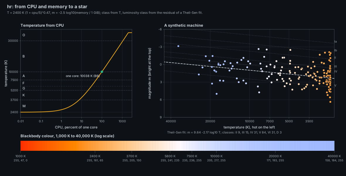
Script: docs/figures/hr-blackbody-diagram.py, which re-implements the formulas of src/hr.rs in Python. A class label sits on the faint edge of its band. The fit shown, $m = 9.64 - 2.17\log_{10}T$, belongs to the synthetic population, not to any machine; the demo's much narrower spread of memory gives a nearly flat line (the diagram image above).

Photometry, point spreads and flashes

How a magnitude becomes a star on screen (a sharp core inside a soft halo that grows slowly with brightness), and how births and exits become nova and supernova timelines, is shared with every star-drawing view: see Math: Stellar Photometry. View Ptolemy uses the same magnitude scale for its fixed stars.

Constellations as cgroups

A cgroup is a constellation and a socket link between two processes is a line of its stick figure. Nothing about where a star sits on the dome is measured: the seat is a hash of the process's identity within its cgroup's disc. What is measured is membership (the star is in that cgroup) and the existence and traffic of the line.

Mapping

Visual element	Measured quantity (source)	Transform
Star	a process that is not Kind::Kernel and not a zombie (state Z)	one pickable Frame::star each, at a seat kept until it leaves or changes cgroup
Colour	Process.cpu	$T = 2400(1 + \mathrm{cpu}/5)^{0.47}$ K, cap 40,000 K, through blackbody::color(T, 1.0); the core is mixed 60 % toward white (stellar, CORE_WHITENING)
Size and brightness	Process.memory (RSS; the physical footprint on macOS)	$m$ as above; stellar::spread(shown, frame height), with pixel sizes scaled by height over 720, not by zoom; a bloom Item::Puff when the flux $10^{-0.4(m - 7)}$ is over 60 (a magnitude under 2.55), radius at most 48 px at 1080p
Twinkle	the shared CPU history (History::window), the 10 s before snapshot.elapsed	coefficient of variation CV of a process's CPU, 0 for under 3 readings or a mean under 0.001 %; amplitude $\min(0.8,\ 0.45,\mathrm{CV})$; the sum of three sines at 0.9 to 3.5 Hz with phases from Rng::for_identity, divided by 1.7
Spectral class	$T$	boundaries and subclass above
Luminosity class	residual from the Theil-Sen fit of the sample	thresholds above
Constellation	Process.cgroup (Process.group where the platform has no cgroups); name from Process.group	one layout::Discs disc each, need $\sqrt{\mathrm{capacity} + 3}$
Dashed boundary	the discs	edges between cells of a fixed 64 by 36 grid whose owner is the nearest disc by power distance
Stick figure	Snapshot.links between two stars of one constellation, brightened by Snapshot.link_traffic	a hairline with a gap of $4.5 + 1.6\max(0, 3.5 - m)$ px at each star, brightness $0.35 + 0.65\min(1, \log_{10}(1 + B)/6)$ for $B$ bytes a second, 0.65 with no traffic reading
Link across constellations	Snapshot.links between two constellations	a faint dashed line, up to 360 px (720p) long
Milky Way band	the number of Kind::Kernel processes	intensity $1 - e^{-\mathrm{count}/40}$ (band_strength)
Dust	each kernel thread	one unpickable Item::Puff along the band at a place from its identity hash, whatever the thread does; never on the diagram
Nova	a birth seen between two samples	ramp of brightness over 0.5 s, a burst ring over 1.5 s, and stellar's nova: +4 magnitudes in 0.3 s, e-folding 2 s, over after 6 s
Fade and supernova	an exit (or a zombie)	at most 1 GiB when last seen, a 1.5 s fade; over 1 GiB, a flash to $-6$ in 0.5 s, glow puffs, an expanding blue-to-red shell, over after 8 s
Diagram x	$\log_{10}T$	45,000 K at the left to 2,250 K at the right
Diagram y	$m$	$-6$ at the top to $+9$ at the bottom
Fitted line	the Theil-Sen fit	dashed, with a glow of 36 puffs, over the part of the line inside the window
Labels	the six brightest stars	name K3 III beside the star, in sky and diagram, hidden during a flight
Dome gradient, boundary shapes, seats within a constellation, the Milky Way's shape	none	decorative (the dashed boundaries show membership, not measurements)

How isotop realises it

Module and registry row. src/hr.rs holds Hr (a #[derive(Default)] struct implementing views::ViewModule) and one row of views::REGISTRY: Backdrop::Void, haze: false (pressure haze would tint the dome), flash: false (the view draws its own novae and exits), links: LinkRule::DrawnByView, link_strokes: true, billboard: true, pitch: Some(FRAC_PI_2), keys: "m diagram or sky", a headless warm-up of Phase::Replay over 12 seconds of demo samples under When::DemoHeadless, and the demo options churn and early_giant. It declares no optional Source: cgroups and socket traffic are read for every view and reach the view only through Snapshot::missing. There is no plugin system; the view is compiled in. --hr-diagram sets ViewOptions::hr_diagram, which ViewModule::configure turns into a start in diagram mode.

Per sample and per frame. ViewModule::record calls Hr::observe for every sample, whichever view is shown: it lays out the constellations, seats new stars and keeps a Record per identity (seat, birth and exit times, the three sine waves of its twinkle, and its lag and bend for the flight, all from Rng::for_identity with fixed salts). When hr draws, derive runs once per sample to fit the main sequence (main_sequence, theil_sen), to find where each constellation's name stands and to build the diagram's text, and observe_history reads each star's CV from the shared History once per new sample. The frame itself does the flight, the twinkle and the drawing. The fit leaves out kernel threads, processes under stellar::MEMORY_FLOOR (1 MiB) and stars at either limit of the magnitude range, and above 400 stars (FIT_STARS) uses every k-th star by identity with k = ceil(n / 400). A star's class, label and residual use the newest sample's own temperature and magnitude, the values the fit was made from; its place, colour and size use the eased ones.

The dome is a billboard. A sky place is in sky units, pixels of a 1600 by 900 window at zoom 1. Plot::world maps a sky point to the ground point that appears at that screen offset (Camera::ground of the offset, then the camera centre added), so the dome faces the viewer whatever the rotation and tilt, and pan and zoom apply. The pan is accumulated from the camera centre's moves, each taken at the rotation and tilt of its own frame (Hr::follow, Camera::ground_offset), so turning a panned camera leaves every star on its pixel; after a gap (another view shown) it starts again at the middle. ViewInfo::billboard makes Scene::fit measure the view's bounds under the camera that drew them, not the goal camera, and stage.bounds is the 1600 by 900 window. The dome is one opaque colour field of 288 by 162 nodes (192 by 108 a window, over 1.5 windows: FIELD_NODES, FIELD_SPAN), placed by Placement::Corners from four world corners: a plum glow, a cove of light along the horizon, a vignette, a dark rim that arches across the bottom, and the Milky Way (value noise with a dust lane). The part that never changes (Dome) is built once; the band's strength is added when the kernel-thread count changes, or while a flight changes the sky's opacity, and the field's revision increases.

Constellations and seats. layout::Discs places one disc per constellation, keyed by Process.cgroup (the app group on macOS) with need $\sqrt{\mathrm{capacity}+3}$, where the capacity is 12 or the next of 12 times 1.5 repeatedly (capacity, MIN_CAPACITY, CAPACITY_GROWTH), so a disc is re-placed rarely and a tenth of a population coming and going leaves it where it is. Discs reserves 1.15 times the need. Centres are stretched 1.6 times wider than tall (STRETCH), 24 sky units per unit of need (UNIT), and shrunk to fit 0.92 of the window (FILL); the layout grows back only if it would fit 1.5 times larger (REGROW). A star's seat is a point within 0.85 of its disc (SEAT_RADIUS) from its identity hash, pushed once to at least 1.7 units of need from every star already seated (SEPARATION), then kept. The boundaries come from the 64 by 36 grid and are recomputed only when a disc is placed, grows or arrives, or the layout's scale changes. So stars move only when their constellation changes or when the whole layout is rescaled; the view harness checks that nothing moves when CPU and memory scale or a tenth of the population turns over.

Drawing a star (draw_stars). Faintest drawn first so the brightest stand over their neighbours: a nova burst, a bloom for flux over 60 (strength $\min(0.026,\mathrm{flux}^{0.3}, 0.22)$), then Frame::star with stellar::spread(shown, height).puffed(): a pickable sphere core inside a halo drawn as Item::Puff, which rounds on both rasterizers so that the CPU and GPU backends agree where halos overlap (parity against a GPU was not run here). A star whose core is under 2.5 px gets a pick-only disc (PICK_RADIUS). shown is the magnitude less the twinkle, Stage::growth and a nova's brightening: $m - 2.5\log_{10}(\mathrm{brightness})$. Stick figures are hairline_between strokes with a gap that shrinks with magnitude; Stage::links (key c) chooses all, only the highlighted, or none.

The flight. m reaches ViewModule::key as ViewKey::Local('m') and sets a flag that the next draw turns into Mode::toggle, from wherever the flight is. A whole crossing takes 1.5 s of Stage::time (TRANSITION_SECONDS), linear in progress. Each star follows a quadratic Bezier from its seat to its diagram place, bent sideways by up to 0.25 of its length (MAX_BEND), with the cubic in-out ease (ease) applied after a lag of up to 0.28 (MAX_LAG) that is stretched so every star arrives at progress 1: a star waits half its lag and then eases over what is left. At progress 0 and 1 the star is exactly at its seat or its diagram place. The sky fades with $1 - \mathrm{smoothstep}(0, 0.62, p)$, the diagram comes up with $\mathrm{smoothstep}(0.38, 1, p)$, and twinkle fades to 30 % of itself on the diagram. A star's diagram place (diagram_position) is a pure function of its own temperature and magnitude; the mode is state of the view, kept by the scene.

Births and exits. The view detects them itself from consecutive samples (Record::born, Record::left), not from Snapshot.life: a process first seen after the first sample is a nova; one that vanishes (or becomes a zombie) while it last held more than 1 GiB (stellar::exit_flash) goes supernova, below that it fades. Exits are remembered for 10 s (RECORD_KEEP) and drawn where the star stood in whatever mode and flight the frame is in. Going back in time (a rewind) forgets events. The demo's early_giant option, with churn, brings the first exit of a process above 1 GiB forward to demo second 8.8 (DEMO_EARLY_KILL), so that a supernova shell is on screen at --time 12.

Text. Labels use Stage::tags (a text beside a point, Side::Right), so they stay off the star: the six brightest stars (LABELLED) as name and class. stage.places holds the constellation names (each in the clearest part of its disc, kept while that spot stays 0.8 as clear as the best) or, once a flight has landed on the diagram, its text: the title, O B A F G K M, the temperature ticks with the CPU that makes them, the magnitude ticks with the memory each stands for, and the regions main sequence, giants, supergiants and white dwarfs where the fit puts them. The inspector lines (stage.notes) read class K3 III | T 4604 K | m +1.23, main sequence m ... | residual ... and CPU variation (CV) ... over 10 s | twinkle ...%. The tour and the Space visits go to the twelve brightest stars (TOURED). Every name goes through label_name and the existing sanitizer. Kernel threads have no star, so while the sky is shown stage.positions records their dust places, for search and the tour.

Legend. In the sky: N stars | K kernel threads in the Milky Way | C constellations | colour = blackbody T = 2400 K x (1 + cpu/5)^0.47 | ... | m diagram. In the diagram: N stars | main sequence m = a - b log T | x = temperature ... | m sky. With | no cgroups: constellations = app groups and | no socket traffic: lines at one brightness appended when those sources are missing (status::missing_note).

Platforms. Linux: everything above. macOS: available; there are no cgroups, so constellations are the app groups (Process.group) and the Milky Way holds kernel_task; where socket links have no traffic reading the figures are drawn at one brightness and the legend says so (which of these applies on a given Mac was not run here: unverified).

Compared with the mockups. The reference mockups were rendered by docs/mockups/code/hr.py from synthetic data and fixed the look the view was built to (the mockup's toggle key was d, which pans in isotop, so the view uses m):

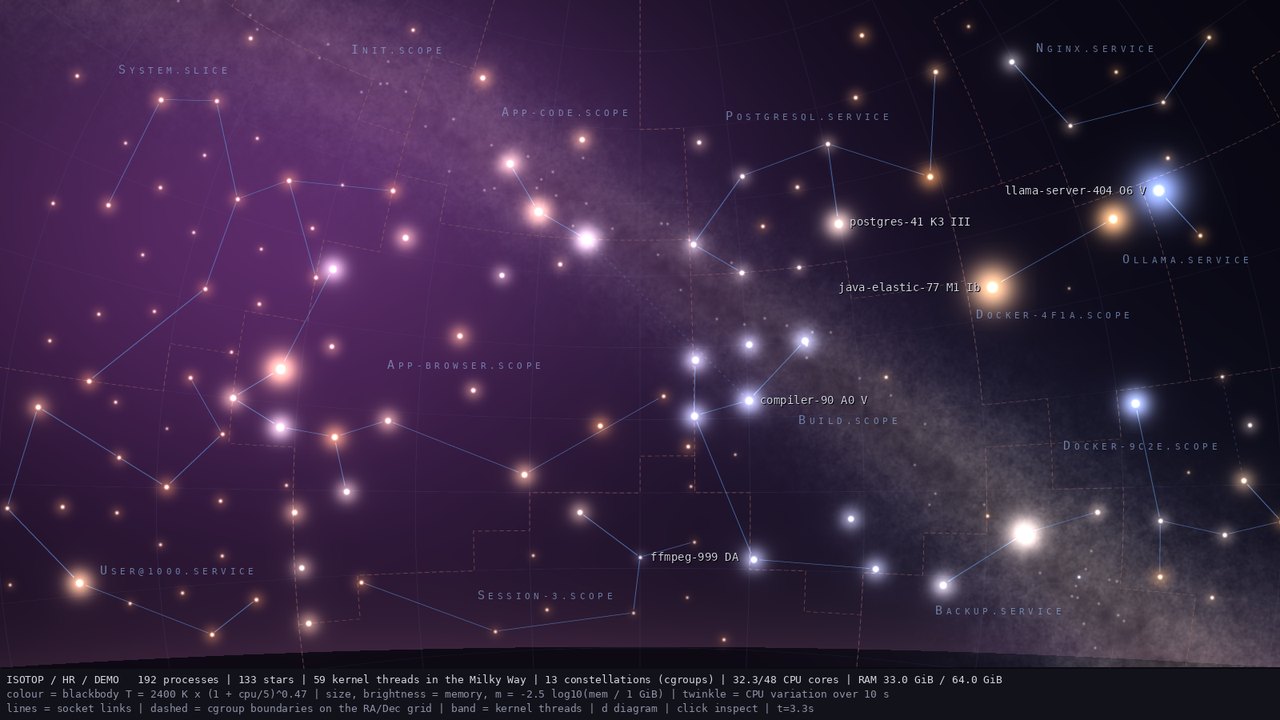
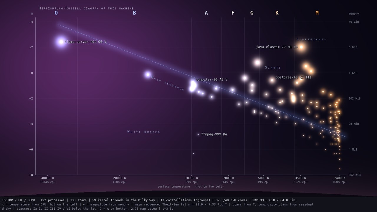
The mockup diagram has a steep main sequence (its status line gives a fit of $m = 29.6 - 7.33\log T$) with giants above it and a white dwarf below. The demo's processes hold a narrow range of memory, so its sequence is nearly flat, and a real machine, where memory runs over several orders of magnitude, is nearer the mockup.

Reading the picture

• Colour is CPU, brightness is memory, and they are independent. The hue encodes one number, the brightness another. The blackbody table is normalised to its brightest channel, so a hot dim star has the same brightness range as a hot bright one.
• Class letters are CPU bins; the digit is a position within the bin. A0 says only that CPU is just under one core; one core is B9. An idle process is M9 whatever its memory. The luminosity class is relative to this machine's own fit, so a "giant" on a quiet machine and a "giant" on a busy one are different things: it says "unusually large for its CPU". As an example with a hypothetical fit at $m = +1.5$, an idle 8 GiB process ($m = -2.26$) has residual $-3.76$ and is M9 II; a K3 III is a star at about 15 % CPU. The class changes with the fit, and the fit changes with the sample.
• Twinkle is a variability measure, not scintillation. Its amplitude is the CV of CPU over 10 s; a perfectly steady process does not twinkle at any CPU level, one with fewer than three samples in the window does not either, and the amplitude is capped at 0.8.
• Sky position is not data. Which part of a constellation a star sits in tells nothing; whether it is in the constellation does. The pattern changes only when a disc is placed or grows, or the layout is rescaled.
• Stick figures show socket links inside a cgroup; a missing line does not prove two processes do not talk (unreadable processes, pipes, shared files). Brightness is the link's measured rate where there is one, not the number of sockets.
• The Milky Way is a count. Kernel threads are drawn as unresolved light and their count sets the brightness; they are not on the diagram, and no thread is distinguished from another.
• Limits. The clamps hide differences: 251 GiB and above is one magnitude, every process under 1 MiB is another ($+7.53$), and everything above about twenty cores is 40,000 K. Under about 4 MiB (magnitude +6) a star has no halo, only a core (see Math: Stellar Photometry). The diagram's top and bottom edges are where stars saturate, not where the data ends.
• The fit is the machine's, not nature's. It is a line of $m$ on $\log T$ whatever the real shape; with under three usable points there is none and no luminosity class is drawn.

Try it

Commands run with the release binary on Linux (x86_64, CPU renderer), repository root:

./target/release/isotop --list-views
./target/release/isotop --demo --view hr --time 12 --width 1600 --renderer cpu --output /tmp/hr-sky.png
./target/release/isotop --demo --view hr --time 12 --hr-diagram --width 1600 --renderer cpu --output /tmp/hr-diagram.png

The first lists twenty-one views, hr after arbor. The second wrote 1600x900, 211 visible (the stars and the kernel threads of the dust) and the third 1600x900, 163 visible (the stars alone: the dust is not on the diagram). Live: ./target/release/isotop --view hr, or Tab and the v picker; m flies between the sky and the diagram, c cycles the links, and Space visits the brightest stars. The figure regenerates with python3 docs/figures/hr-blackbody-diagram.py.

Where in the code

Item	Path and symbol
The view	src/hr.rs: Hr, temperature, star_magnitude, spectral_class, luminosity_class, classification, theil_sen, main_sequence, Fit, variation, twinkle_amplitude, diagram_position, flight, Mode, Record, Dome, band_strength, link_brightness, Plot
Registry row	src/views.rs: REGISTRY row hr; ViewOptions (hr_diagram) and ViewModule::configure
Flag	src/main.rs: --hr-diagram
Stars and flashes	src/stellar.rs: magnitude, MEMORY_FLOOR, spread, Frame::star, Flash, exit_flash, flash
Colour	src/blackbody.rs: TABLE, linear, color
Dome field	src/render/field.rs: Field, Placement::Corners
Shared helpers	layout::Discs, simulation::Rng::for_identity, History::window, Stage::growth, Stage::tags, Camera::ground, status::missing_note
Figure	docs/figures/hr-blackbody-diagram.py
Prototype (reference only)	docs/mockups/code/hr.py
Related pages	Math: Stellar Photometry, Theory: Colour, Theory: Stable Layout, View Ptolemy, View Horizon

Variations and open questions

• Isochrones and tracks. Draw each process's last minute of $(T, m)$ as a path on the diagram, as astronomers draw evolutionary tracks, from the shared history.
• A mass-luminosity analogue. The legend already prints the fit's slope; plot it over time, as the exponent in $L \propto M^{3.5}$ is reported for stars, and ask whether it is stable across machines.
• Clusters. The Pleiades and Hyades are clusters at a common distance, which is what made Hertzsprung's diagram work. A cgroup is the equivalent: fit and plot one cgroup alone and see whether it has a sequence of its own.
• Colour-blind safe palette. The only measured encoding in hue is temperature; issue #104 (colour-blind safe palette) has to decide what to do with a hue-only variable.
• Bolometric corrections. Stars are drawn at their bolometric magnitude, not by band; a "V-band" variant would dim very hot and very cool stars by the bolometric correction.
• The observer's class. If isotop is listed among the processes it is classified like any other: about B9 at one core, M when idle. Which a viewer sees depends on whether the frame loop is the hottest thing on the machine.
• Dust. Interstellar reddening could be a metaphor for memory pressure: pressure shifts colours toward red. The row turns haze off for now.
• A moving seat. Seats are frozen so the sky is stable; a variant could let the members of a cgroup drift toward their communication partners and measure what stability costs.

References

• H. N. Russell, "Relations between the spectra and other characteristics of the stars", Nature 93, 252-258 (1914) (as the Linda Hall Library lists it); also in Popular Astronomy 22, 275 and 331 (1914) (pages from memory).
• E. Hertzsprung, "Zur Strahlung der Sterne", Zeitschrift für wissenschaftliche Photographie 3, 429 (1905) and 5, 86 (1907) (pages from memory).
• A. C. Maury and E. C. Pickering, "Spectra of bright stars photographed with the 11-inch Draper telescope as a part of the Henry Draper Memorial", Annals of Harvard College Observatory 28, part 1 (1897).
• A. J. Cannon and E. C. Pickering, The Henry Draper Catalogue, Annals of Harvard College Observatory 91 to 99 (1918 to 1924).
• H. S. Leavitt and E. C. Pickering, "Periods of 25 variable stars in the Small Magellanic Cloud", Harvard College Observatory Circular 173 (1912).
• M. N. Saha, "Ionization in the solar chromosphere", Philosophical Magazine 40, 472 (1920); C. H. Payne, Stellar Atmospheres, Harvard Observatory Monographs 1 (1925); H. N. Russell, "On the composition of the Sun's atmosphere", Astrophysical Journal 70, 11 (1929).
• W. W. Morgan, P. C. Keenan, E. Kellman, An Atlas of Stellar Spectra, with an Outline of Spectral Classification, University of Chicago Press (1943); W. W. Morgan and P. C. Keenan, "Spectral classification", Annual Review of Astronomy and Astrophysics 11, 29 (1973).
• A. S. Eddington, "On the relation between the masses and luminosities of the stars", Monthly Notices of the Royal Astronomical Society 84, 308 (1924) (pages from memory); H. A. Bethe, "Energy production in stars", Physical Review 55, 434 (1939).
• S. Chandrasekhar, "The maximum mass of ideal white dwarfs", Astrophysical Journal 74, 81 (1931); E. M. Sion et al., "A proposed new white dwarf spectral classification system", Astrophysical Journal 269, 253 (1983) (pages from memory).
• N. R. Pogson, "Magnitudes of thirty-six of the minor planets for the first day of each month of the year 1857", Monthly Notices of the Royal Astronomical Society 17, 12 (1856).
• C. Wyman, P.-P. Sloan, P. Shirley, "Simple analytic approximations to the CIE XYZ color matching functions", Journal of Computer Graphics Techniques 2(2), 1-11 (2013); M. Charity, "What color is a blackbody?", http://www.vendian.org/mncharity/dir3/blackbody/ (the address the tests of src/blackbody.rs give; not fetched here); the CIE 1931 colour matching functions and the sRGB standard (IEC 61966-2-1).
• H. Theil, "A rank-invariant method of linear and polynomial regression analysis", Nederlandse Akademie van Wetenschappen Proceedings 53, 386 (1950) (pages from memory); P. K. Sen, "Estimates of the regression coefficient based on Kendall's tau", Journal of the American Statistical Association 63, 1379 (1968).
• E. Delporte, Délimitation scientifique des constellations, Cambridge University Press (1930); H. A. Rey, The Stars: A New Way to See Them, Houghton Mifflin (1952); D. Sobel, The Glass Universe, Viking (2016); C. Payne-Gaposchkin, The Galactic Novae, North-Holland (1957).
• IAU 2015 Resolution B2, on zero points for the absolute and apparent bolometric magnitude scales.