Theory Simulation Toolkit

Theory: The simulation toolkit

src/simulation.rs is the one file of shared, pure numerical helpers: neighbour queries over 2-D and 3-D points, a seeded random generator with a Gaussian, hashes, a complex type with a direct and a fast Fourier transform, a fixed-step clock, and the easing functions. "Nothing here draws or reads the system." This page states each tool as mathematics first, then as the code does it, with the properties the tests pin and the numbers that go with them. The hashing and seeding are developed on Determinism, the grid on Spatial hashing, the epicycle application of the DFT on Fourier epicycles, and the placement helpers on Stable layout.

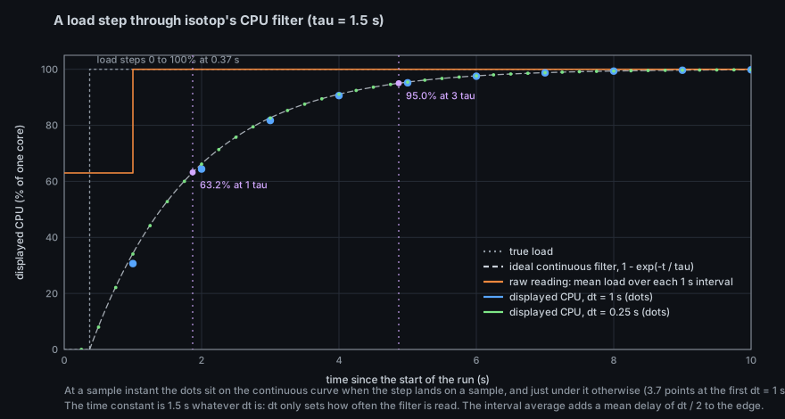
The exponential smoother of section 6.3, here as the CPU pipeline uses it (time constant 1.5 s). See Model and rates.

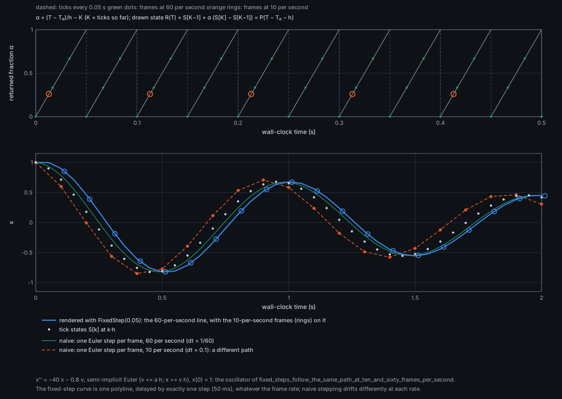
The fixed-step clock of section 5 with step = 0.05 s. Top: ticks (dashes) and frames at 10 and 60 per second; the saw-tooth is the returned fraction. Bottom: the damped oscillator of the unit test, its tick states, and the rendered position at 10 and 60 frames per second: all on one curve.

The rule that makes a toolkit necessary is in AGENTS.md: "Shared helpers live in one place each. Don't write a second copy." A test (no_hand_rolled_hashes_outside_simulation) enforces it for the hash and random constants by scanning every other source file. It does not (yet) cover the easing helpers; see "Duplicates" in section 8.

History

Most of this file is older than the computers it runs on. The fast Fourier transform is the clearest case. Cooley and Tukey published the algorithm in Mathematics of Computation in 1965, and it is usually told as the moment the discrete Fourier transform fell from $N^2$ operations to $N\log N$. Heideman, Johnson and Burrus (1985, Archive for History of Exact Sciences 34) found the same decomposition in an unpublished manuscript of Gauss, presumably written in 1805, before Fourier presented his harmonic analysis in 1807. Gauss was interpolating the orbits of the asteroids Pallas and Juno from a handful of observations. The manuscript appeared only in his collected works, in 1866 (volume 3).

The Gaussian generator is from 1958, when Box and Muller (Annals of Mathematical Statistics 29(2)) showed that two uniform deviates become two independent normal ones through a logarithm and a rotation. Marsaglia and Bray's polar method (SIAM Review 6, 1964) removes the trigonometry at the price of a random, rejected number of uniform draws, which section 2 gives as the reason the code does not use it. The exponential smoother that smoothing discretises has a military origin. Robert G. Brown, an operations analyst for the US Navy, built a tracking filter of this kind for antisubmarine fire control in 1944; in the early 1950s he applied it to demand for spare parts, because it needed one stored number per item where a moving average needed a window, and presented the inventory work in 1956 (his book on inventory control is dated 1959; sources differ on which counts as the beginning). Charles Holt arrived at exponentially weighted averages independently in a 1957 Office of Naval Research report that was not formally published until 2004.

Fixed-step simulation became a recognised idiom through game programming; Fiedler's "Fix Your Timestep!" (the reference list dates it 2004) is the usual citation, and the constants of FixedStep, a step, a cap on steps per frame and a cap on the gap, are that article's "semi-fixed" safeguards written as parameters. Uniform grids for neighbour queries are standard in collision detection (Ericson 2005); Bentley's k-d tree (1975) is the alternative the spatial-hashing page compares them with. The splitmix64 and xorshift generators, and the FNV hash, have their histories on Determinism.

1. Summary table

tool	what	cost	production callers
SpatialHash	uniform grid, radius query in 2-D	build $O(n\log n)$; query $\approx(2r/s+1)^2$ cells plus their points	Coop (NEIGHBOURHOOD = 4)
SpatialHash3	the same in 3-D, plus exact $k$-nearest	build $O(n\log n)$; $k$-nearest one or two shells of cells	Murmuration (nearest)
Rng	splitmix64; unit, signed, normal	one 64-bit add and finaliser per draw	Necropolis, Ptolemy, Coop, Murmuration, Arbor, Cortex, Horizon, model (demo)
hash_identity, Rng::for_identity	seed from pid, start time, salt	three finaliser rounds	same
XorShift32	Marsaglia xorshift, shifts (13, 17, 5)	three shifts and xors	Flow
hash::*	legacy bit-exact hashes, FNV-1a	few ops	many views, golden test
Complex, dft	direct DFT, any length	$O(N^2)$ in f64	Ptolemy (60 samples)
fft, inverse_fft	radix-2 Cooley-Tukey	$\tfrac N2\log_2 N$ butterflies	none yet
FixedStep	whole-step clock with interpolation fraction	$O(\text{steps})$	Coop (0.05, 10, 0.5), Arbor, Murmuration, Cortex
growth, sprout, smoothing, smoothstep	easing	a few flops	most views

fft and inverse_fft (with their helpers require_power_of_two and transform) carry #[cfg_attr(not(test), expect(dead_code, reason = "no caller until the first view that uses it"))], and SpatialHash3::neighbours the same with its own reason ("no caller until a view that needs a radius query"). They were built ahead of the views that need them (building block P4, #20) and are exercised by tests only. SpatialHash3::nearest and Rng::normal, which carried the marker until Murmuration and Horizon arrived, are in production use.

2. Rng and the hashes

Rng is splitmix64 (state, += 0x9e3779b97f4a7c15, three-step finaliser). unit() is (next_u64() >> 40) as f32 / 16_777_216.0, uniform on ${k/2^{24}}$, in $[0,1)$; signed() is unit() * 2 - 1 in $[-1,1)$. The derivations, the seeding by hash_identity(id, salt) and the legacy hash:: functions are on Determinism; here is the one that has a mathematical content of its own.

Rng::normal

Rng::normal is the Box-Muller transform (Box and Muller 1958), in its trigonometric form, discarding the second value of each pair:

let radius = (-2.0 * (1.0 - self.unit()).ln()).sqrt();
radius * (std::f32::consts::TAU * self.unit()).cos()

If $U_1,U_2$ are independent and uniform on $(0,1]$ and $(0,1)$, then $R=\sqrt{-2\ln U_1}$ and $\Theta=2\pi U_2$ give $(R\cos\Theta,,R\sin\Theta)$ with two independent standard normal coordinates. The proof is two lines. $P(R>r)=P(U_1<e^{-r^2/2})=e^{-r^2/2}$, so $R$ has density $re^{-r^2/2}$; $\Theta$ is uniform and independent of $R$; the density of a point with polar coordinates $(R,\Theta)$ in the plane is therefore $\frac1{2\pi}e^{-r^2/2}$ with respect to $r,dr,d\theta$, which is the bivariate standard normal in Cartesian form, $\frac1{2\pi}e^{-(x^2+y^2)/2},dx,dy$.

Details that are the code's own:

• u1 = 1 - unit() lies in $(0,1]$, so the logarithm never sees zero. Since unit() is a multiple of $2^{-24}$ below 1, 1 - unit() is exact in f32.
• Exactly two uniform draws per call, and no cached half. The second member of the pair ($R\sin\Theta$) is thrown away. That wastes half the transform but keeps the generator a single state word, and, more importantly, keeps stream positions predictable: a view that draws one Gaussian per bird consumes the same number of 64-bit words whatever else happens. The test rng_normal_leaves_the_uniform_stream_alone checks that after one normal() the stream equals the stream after two unit() calls. (Marsaglia's polar method avoids the trigonometry but draws a random, rejected number of uniforms; that would break this property.)
• Truncated tails. The smallest $U_1$ is $2^{-24}$, so $|\text{normal}|\le\sqrt{2\cdot24\ln2}=5.77$. The mass beyond $5.77\sigma$ that is missing is about $8\times10^{-9}$. For layout noise and flocks that is irrelevant; for a rare-event simulation it would not be.
• Test. rng_normal_has_zero_mean_and_unit_variance: 100 000 draws from Rng::new(42), mean within 0.02 of 0 and variance within 0.02 of 1 (the standard errors are 0.003 and 0.0045, so the margin is more than four sigma). rng_normal_is_deterministic_per_seed pins determinism.

3. Complex numbers, dft and fft

Complex { re: f32, im: f32 } with Add, Sub, Mul, norm (hypot), conj, from_angle ($e^{i\theta}$), scale. The transforms use one convention, fixed in the doc comments and in a test:

$$ X[k]=\sum_{n=0}^{N-1}x[n],e^{-2\pi i kn/N},\qquad x[n]=\frac1N\sum_{k=0}^{N-1}X[k],e^{+2\pi i kn/N}. $$

The forward transform is unscaled and uses the negative exponent; the inverse carries the $1/N$ and the positive exponent. Consequences worth having in one place: a pure tone $x[n]=e^{+2\pi i k_0 n/N}$ transforms to $X[k]=N,\delta_{k,k_0}$; a real sine at bin 1 transforms to $X[1]=-iN/2$ and $X[N-1]=+iN/2$ (the test fft_follows_the_negative_exponent_convention checks exactly these, $-4$ and $+4$ at $N=8$); Parseval reads $\sum|x|^2=\frac1N\sum|X|^2$.

3.1 dft

The direct sum, $O(N^2)$, for any length (the Ptolemy view transforms 60 samples and would need padding for a radix-2 FFT). Twiddles and sums are f64, only the result is rounded to f32. The angle is formed from $(kn\bmod N)/N$ rather than $kn$, which keeps the argument of sin_cos in $[0,1)$ turns and the rounding error small for large $kn$. It is the reference the fast transform is tested against. Cost for $N=60$: 3 600 complex multiply-adds.

3.2 fft: radix-2 decimation in time

Split $x$ into even- and odd-indexed halves. With $W_N=e^{-2\pi i/N}$ and the half-size transforms $E,O$:

$$ X[k]=E[k]+W_N^{k},O[k],\qquad X[k+N/2]=E[k]-W_N^{k},O[k],\qquad 0\le k<N/2 , $$

because $W_N^{k+N/2}=-W_N^k$. Recursing gives $\log_2N$ stages of $N/2$ such butterflies: $\tfrac N2\log_2N$ complex multiplies, 5 120 at $N=1024$ against 1 048 576 for the direct sum, a factor of 205. The code is the iterative form:

1. Bit reversal: partner = index.reverse_bits() >> (usize::BITS - length.trailing_zeros()), swapped when partner > index. This puts the even/odd recursion's leaves in order.
2. Twiddle table of $N/2$ entries $W_N^{j}$, computed in f64 and rounded once to f32, so the error grows with the $\log_2N$ rounding steps of the butterflies rather than with the angle error of an f32 recurrence.
3. Stages: half = 1, 2, 4, ...; a stage spans 2 * half and uses every stride = length / (2 * half)-th table entry; each butterfly reads buffer[start+offset] and buffer[start+offset+half] * twiddles[offset*stride].

The length must be a power of two; anything else panics, naming the length (require_power_of_two, tests fft_panics_on_a_length_that_is_not_a_power_of_two). Length 0 and 1 are the identity. The accuracy test compares against dft for every power of two up to 1024 with a relative error bound of $10^{-5}$ (about $10^{-6}$ measured at $N=1024$).

inverse_fft uses the conjugation identity

$$ \mathrm{IDFT}(X)=\frac1N,\overline{\mathrm{DFT}(\overline X)} , $$

conjugate, run the forward transform, conjugate and scale by $1/N$, so there is one transform to get right. Test: inverse_fft_restores_the_input for lengths 2, 16, 256, 1024.

Application: a closed curve sampled as $z[n]=x[n]+iy[n]$ has coefficients $X[k]$ that are circles of radius $|X[k]|/N$ turning at $k$ turns per period: this is the epicycle decomposition of Ptolemy (Fourier epicycles).

4. SpatialHash and SpatialHash3

The mathematics (expected cost, the choice of cell size, the exactness argument for the shell search, degenerate distributions, the comparison with trees) is on Spatial hashing. The interface, as the code states it:

• new(cell): non-positive or non-finite sizes fall back to 1.
• rebuild(points): replaces the points, reusing allocations (a test checks the buffers keep their capacity at a steady count). One sort of point indices by (cell key, index); a map from cell key to (start, end).
• neighbours(point, radius, out): indices of stored points at distance strictly less than radius, in ascending index order; a stored query point is included at distance zero. radius NaN, zero or negative gives an empty result. When the query box covers more cells than there are points, it scans all points instead.
• SpatialHash3::nearest(point, k, out): the exact k nearest as (index, distance) sorted by distance and then index; k larger than the count returns everything; the query point itself is at distance 0 and the caller filters it.

Two implementation details are instructive. The sort key of a (index, distance) candidate is one integer, u64::from(distance.to_bits()) << 32 | index: the bit pattern of a non-negative f32 orders like its value, and a NaN (bits above $+\infty$) ranks after every number, so sorting integers sorts by distance, then index, with NaN last. And the 3-D grid hashes a cell with its own CellHasher (a multiply and a fold of the high half onto the low) rather than SipHash, which "cost a k-nearest query about as much as the distances it computes".

5. FixedStep: a clock that makes every frame rate follow one trajectory

5.1 The problem

A simulation advanced by the time since the last frame, $x\leftarrow F(x,\Delta t)$, follows a different trajectory at each frame rate whenever $F$ is not exactly composable: $F(F(x,\tfrac12\Delta),\tfrac12\Delta)\ne F(x,\Delta)$ for explicit Euler, collision responses, stochastic updates, anything with a threshold. 10 and 60 frames per second then show different worlds, and a stall or a pause becomes a huge $\Delta t$ that throws the state out of its stable region. The cure (Fiedler 2004, "Fix Your Timestep!") is to advance the simulation in fixed steps $h$ and let the frame rate only decide how many steps happen to be due, then interpolate the drawn state between the last two.

5.2 The algorithm, exactly as coded

FixedStep::new(step, max_steps, max_gap) holds clock: Option<f32> (last time seen) and accumulator. One call advance(time, tick) -> f32:

dt = (time - last).min(max_gap)   if a last time exists and time >= last,   else 0
clock = time
accumulator += dt
steps = 0
while accumulator >= step and steps < max_steps:  tick(step); accumulator -= step; steps += 1
accumulator = min(accumulator, step)              # drop any backlog beyond one step
return clamp(accumulator / step, 0, 1)

The first call, a repeated time and a time that went back (a rewind) take no steps; after a rewind the clock resumes from the new time (tested). A paused scene feeds the same stage.time and so takes none.

5.3 What the interpolation fraction is

Let $T_0$ be the clock's first time, $T$ the current one, and assume no clamp has acted. After the call the accumulator holds exactly the time not yet turned into steps. Invariant: $a=(T-T_0)-hK$, where $K$ is the number of ticks taken so far, and the loop keeps $0\le a&lt;h$. Hence

$$ K=\Bigl\lfloor\frac{T-T_0}{h}\Bigr\rfloor ,\qquad \alpha=\frac ah=\frac{T-T_0}{h}-K\in[0,1). $$

The tick count depends on the clock time alone, not on how the frames fall: partition the interval into 10 or 60 frames per second and the loop executes the same ticks, in the same order, with the same step. That is the "same path" property, tested by fixed_steps_follow_the_same_path_at_ten_and_sixty_frames_per_second (a damped oscillator integrated at 10 and at 60 frames per second, three seconds, FixedStep::new(0.05, 10, 0.5): the states at every step count that both runs reach are bitwise equal, at least 25 of them) and by Coop's flock_follows_the_same_path_at_ten_and_sixty_frames_per_second. The test compares states at equal step counts, not at equal frame times, because f32 accumulation can shift a tick across a frame boundary by one.

The returned $\alpha$ is how far the frame lies into the next step. With $S_{K-1}$ and $S_K$ the last two tick states (Coop keeps previous and position per chicken and draws previous + (position - previous) * alpha), the drawn state is

$$ R(T)=S_{K-1}+\alpha,(S_K-S_{K-1}) , $$

which is the value at time $(K-1+\alpha)h=T-T_0-h$ of the piecewise-linear interpolant $P$ through the points $(kh,S_k)$. So

$$ R(T)=P(T-T_0-h). $$

The rendered motion is a function of the clock time alone, delayed by exactly one step, whatever the frame rate: frames at 10 and 60 per second sample the same curve. That is the bottom panel of the figure. The price is the delay: 50 ms for Coop's $h=0.05$, half a frame at 10 frames per second and invisible. (Drawing $P(T-T_0)$ would require the next state, which does not exist yet; extrapolating instead of interpolating removes the delay and brings back the frame-rate-dependent error.)

5.4 The spiral of death and the two caps

Let a tick cost wall-clock time $c$. A frame that is $\Delta$ seconds late must run $\Delta/h$ ticks, which takes $c\Delta/h$. If $c&gt;h$ that is more than the time being caught up, so the next frame is later still, and the work per frame diverges. Two parameters prevent it:

• max_gap bounds the time a single call counts, dt.min(max_gap): a long stall (a suspended laptop, a debugger breakpoint, a pause) is dropped instead of simulated. Simulation time then lags wall-clock time permanently by the dropped part, which is the right behaviour for a visualization.
• max_steps bounds the work of one call. With max_steps * step >= max_gap (Coop: $10\times0.05=0.5$) the second cap is the first cap seen from the other side; with a smaller max_steps the call may leave more than a step in the accumulator, and the final accumulator.min(step) discards the excess so it cannot pile up (test a_long_stall_runs_at_most_max_steps_and_drops_the_rest: a 10 s stall with max_gap 100 and 10 steps runs 10 ticks, keeps one backlog step, and the next 0.01 s completes it and nothing more).

When the cap is hit, the fraction is exactly 1 (the clamp of the final min). The steady-state condition for real-time simulation is $c&lt;h$ per tick, so the simulation costs under one wall-clock second per simulated second; the catch-up capacity of Coop is max_steps * step = 0.5 simulated seconds per frame, five times real time at 10 frames per second.

5.5 Relationship to Stage::dt

render.rs computes a second, simpler policy for all views: FrameClock::step(time, paused) is 0 on the first frame, while paused and when time <= last; otherwise min(time - last, MAX_DT) with MAX_DT = 0.5. It differs from FixedStep in two ways: it hands out a variable step, and it uses a strict comparison (time > last) where FixedStep accepts time >= last (equal times add zero anyway). Use stage.dt for anything that integrates a smooth, composable flow (the exponential easings below are composable, so they are safe); use FixedStep for anything that is not. docs/VIEW_CONVENTIONS.md says to choose the step $H$ per view, state it in the README, and prove with a 10 versus 60 frames per second test.

6. Easing: four functions and their properties

6.1 growth and sprout: a cubic ease-out

pub const GROW_SECONDS: f32 = 0.9;
pub fn growth(births, id, time) -> f32 {
    let born = births.get(&id).copied().unwrap_or(f32::NEG_INFINITY);
    if time < born { return 1.0; }
    let t = ((time - born) / GROW_SECONDS).min(1.0);
    1.0 - (1.0 - t).powi(3)
}
pub fn sprout(growth: f32) -> f32 { 0.3 + 0.7 * growth }

$$ g(t)=1-(1-t)^3,\quad g'(t)=3(1-t)^2,\quad g''(t)=-6(1-t),\quad t=\min\Bigl(\frac{\text{time}-\text{born}}{0.9},1\Bigr). $$

$g(0)=0$, $g(1)=1$, $g$ is increasing, with its fastest speed $g'(0)=3/0.9=3.33$ per second at birth and a smooth landing: $g'(1)=g''(1)=0$, so the joint with the constant 1 after $t=1$ is $C^2$. A new process therefore bursts out and settles, which reads as "arrival". A process with no recorded birth, or born in the future, is fully grown (1.0), so headless frames and rewinds show everything grown. sprout(g) maps the growth to a size scale in $[0.3,1]$, "so a newborn is small but never a speck". Both are stateless in time: pure functions of (birth, now), computed fresh each frame, which is the form the conventions ask for ("compute closed-form animation from state and time, do not accumulate it per frame").

6.2 smoothstep

$$ S(x)=3x^2-2x^3,\quad x\leftarrow\mathrm{clamp}(x,0,1),\qquad S'(x)=6x(1-x),\quad S''(x)=6-12x . $$

$S(0)=0$, $S(1)=1$, $S'(0)=S'(1)=0$ ("no speed at either end"), $S(\tfrac12)=\tfrac12$, the antisymmetry $S(1-x)=1-S(x)$, and a maximum slope $S'(\tfrac12)=\tfrac32$. It is $C^1$ but not $C^2$ ($S''=\pm6$ at the ends), so the acceleration jumps at the start and end; the quintic $6x^5-15x^4+10x^3$ would remove that and is not in the tree. Used for fades and row openings (Necropolis ROW_EASE, the lift of a risen ghost), for Arbor's blossoms and for Horizon's orbit easing, and for Ptolemy's re-sort ease, whose angle integrates the eased rate (see the comment on its epoch).

6.3 smoothing: the exact discretisation of a first-order low-pass

pub fn smoothing(dt: f32, tau: f32) -> f32 { 1.0 - (-dt / tau).exp() }
//  value += smoothing(dt, tau) * (target - value)

The continuous system $\dot v=(u-v)/\tau$ with the input $u$ held constant over a step of length $\Delta t$ has the exact solution $v(t+\Delta t)=u+(v(t)-u),e^{-\Delta t/\tau}$, i.e. $v\leftarrow v+w,(u-v)$ with $w=1-e^{-\Delta t/\tau}$. This is not Euler's $w=\Delta t/\tau$ (which exceeds 1 and oscillates for $\Delta t&gt;2\tau$) but the exact flow, so:

• $0\le w&lt;1$ for every $\Delta t\ge0$, and $w\to1$ as $\Delta t/\tau\to\infty$: stable for any frame time.
• Composable: $1-(1-w(\Delta_1))(1-w(\Delta_2))=1-e^{-(\Delta_1+\Delta_2)/\tau}=w(\Delta_1+\Delta_2)$. Two half-length steps equal one full step when the target is constant; this is the frame-rate independence of an exponential ease, and what the_orientation_eases_alike_at_ten_and_sixty_frames_per_second checks (agreement within $10^{-3}$ rad after two seconds).
• The step response is $1-e^{-t/\tau}$: 63.2 percent at $t=\tau$, 95.0 percent at $3\tau$; the corner frequency is $f_c=1/(2\pi\tau)$ (0.106 Hz for $\tau=1.5$ s, 0.53 Hz for 0.3 s, 0.80 Hz for 0.2 s).
• For small steps $w\approx\Delta t/\tau$. At the default 1 s sample and $\tau=1.5$ s, $w=0.487$.

Uses in the tree: the collector's CPU smoothing (smoothing(dt, 1.5), with $\Delta t$ the sample interval), Scene::ease for every process's CPU and memory (smoothing(dt, 0.3) with the frame gap, resetting the table if the gap is outside $[0,2]$ s), Horizon's pressure and orbit easing, and the camera (smoothing(elapsed, 0.2) in CameraController::approach, which Camera::approach applies to the centre, rotation and pitch additively and to the zoom as $\text{zoom}\leftarrow\text{zoom}, (\text{goal}/\text{zoom})^{w}$, so the zoom eases exponentially in its logarithm).

A negative dt gives a negative weight, which extrapolates away from the target; Scene::ease guards with dt.max(0.0).

7. Try it

cargo test -p isotop simulation::        # all of the above, including the FFT accuracy sweep
cargo test --release -- --ignored --nocapture timing_nearest_22_of_8000    # nearest k=22 x 8000, fft 1024
./target/release/isotop --demo --view coop --width 960 --renderer cpu --time 30 --output coop.png
python3 docs/figures/simulation-fixedstep.py     # regenerate the figure from the repository root

timing_nearest_22_of_8000_flock_points_and_fft_1024 is #[ignore] (timing; run in release) and asserts under 10 ms for the 8 000 queries; it prints fft 1024 in microseconds.

8. Where in the code, and duplicates

All in src/simulation.rs: growth, sprout, smoothing, smoothstep, Complex, dft, fft, inverse_fft, transform, SpatialHash, SpatialHash3 (rebuild, neighbours, nearest, visit_shell, face_distance), Rng, hash_identity, FixedStep, XorShift32, hash. Users: coop/sim.rs (YardClock, SpatialHash), murmuration.rs (SpatialHash3, FixedStep, Rng), arbor.rs and cortex.rs (FixedStep), ptolemy.rs (dft, smoothstep), necropolis.rs (smoothstep), render.rs (FrameClock, growth, smoothing), model.rs (smoothing, demo Rngs).

Duplicates that contradict the rule. simulation::smoothstep exists, yet the same polynomial is written out again in tesseract.rs (its own fn smoothstep), cores.rs (two inline u * u * (3.0 - 2.0 * u)), coop/creatures.rs (a closure ease), horizon/disk.rs (a closure smooth), horizon/lens.rs (the taper in the plunge brightness) and the demo workload in model.rs; and 1.0 - (-dt / TURN_EASE).exp() is spelled out in tesseract.rs where smoothing(dt, TURN_EASE) would do, as is Arbor's wind easing (1.0 - (-STEP / WIND_EASING).exp()). They are numerically identical today, so replacing them changes no pixels; no test guards it.

9. Variations and open questions

• A fixed-step Flow. Flow clamps dt to 0.1 s and draws from one shared XorShift32; moving it onto FixedStep with counter-based seeding is the plan in #92.
• A higher-order integrator. The test oscillator is semi-implicit (symplectic) Euler, $v\leftarrow v+a,h,\ x\leftarrow x+v,h$. A leapfrog or velocity-Verlet step with the same h would let h grow by a factor for the same energy drift.
• Real-input FFT. Every use of the transform has real input; a packed real FFT halves the work.
• Waiting for a signal. fft and inverse_fft have no production caller and a test for every power of two up to 1024. Which signal in a process table has a period worth finding is unanswered.
• Marsaglia versus Box-Muller. Compare the cost per normal and the stream-alignment property of the polar method with a fixed-consumption rejection (always draw four uniforms).
• Quintic smoothstep. Replace $3x^2-2x^3$ by the $C^2$ quintic in one view and compare the onset of motion by eye.
• Extrapolation instead of delay. Dead-reckon with the last tick velocity to draw $P(T-T_0)$ and remove the one-step delay, at the price of a visible correction at each tick for fast-turning bodies.

10. References

• Box, G. E. P. and Muller, M. E. 1958. "A note on the generation of random normal deviates." Annals of Mathematical Statistics 29(2): 610-611.
• Cooley, J. W. and Tukey, J. W. 1965. "An algorithm for the machine calculation of complex Fourier series." Mathematics of Computation 19(90): 297-301.
• Steele, G. L. Jr., Lea, D. and Flood, C. H. 2014. "Fast splittable pseudorandom number generators." OOPSLA 2014.
• Marsaglia, G. 2003. "Xorshift RNGs." Journal of Statistical Software 8(14).
• Fiedler, G. 2004. "Fix Your Timestep!" (Gaffer On Games).
• Ericson, C. 2005. Real-Time Collision Detection. Morgan Kaufmann. (Uniform grids, chapter 7.)
• Bentley, J. L. 1975. "Multidimensional binary search trees used for associative searching." Communications of the ACM 18(9): 509-517.