Math Spiking Neurons

Math: Spiking Neurons

A neuron is a leaky capacitor with voltage-gated conductances in parallel, and a spike is what that circuit does when the conductances push back hard enough. In 1952 Alan Hodgkin and Andrew Huxley wrote the circuit down for the squid giant axon in four coupled differential equations; since then the field has spent seventy years deciding how much of it can be thrown away. This page walks that ladder: Hodgkin-Huxley, the leaky integrate-and-fire neuron, and Izhikevich's two-variable model with its table of firing classes, with every trace and number simulated in pure Python (docs/figures/). The Izhikevich model is the engine of the Cortex view, and section 6 says exactly what the code takes from this page.

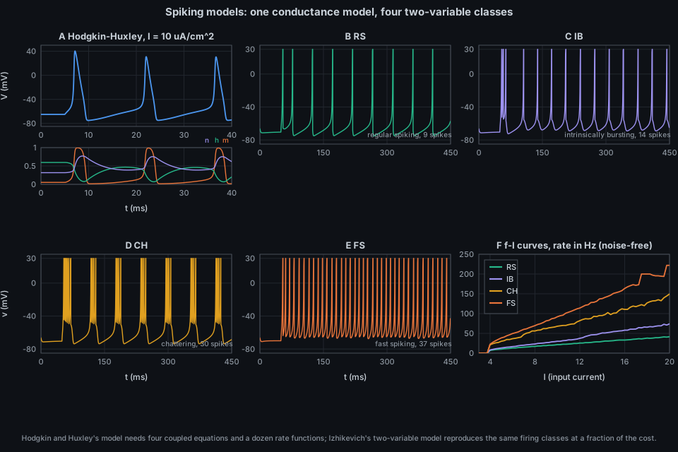
docs/figures/spiking-models.py. A: Hodgkin-Huxley with a 10 uA/cm^2 step, gating variables below. B to E: Izhikevich regular spiking, intrinsically bursting, chattering and fast spiking for a step of $I = 10$ at 50 ms. F: their noise-free f-I curves.

History

The longer account lives in the repository: docs/theory/cortex.md.

The neuron. In the 1880s and 1890s Camillo Golgi's silver stain showed nerve cells whole for the first time, and Santiago Ramon y Cajal used it to argue that the brain is made of separate cells that touch rather than a continuous net. Their opposed interpretations shared the 1906 Nobel Prize in Physiology or Medicine. Cajal's drawings of cortex, with its layers of pyramidal cells, are still reproduced.

The equations. Louis Lapicque (1907) modelled the nerve as a leaky capacitor that fires on reaching a threshold: the integrate-and-fire neuron of section 2, crude and cheap and still in use. Warren McCulloch and Walter Pitts (1943) abstracted the neuron to a threshold logic gate, the root of artificial neural networks. In 1952 Alan Hodgkin and Andrew Huxley, working on the giant axon of the squid at Plymouth and Cambridge, wrote the ionic currents as four coupled equations; they shared the 1963 Nobel Prize in Physiology or Medicine with John Eccles. The numerical solution was done by hand: Huxley integrated the equations on a hand-operated Brunsviga calculator, and by Hodgkin's own account the propagated action potential took about three weeks. The script behind section 1 integrates one spike in about a second. Richard FitzHugh (1961) and Jinichi Nagumo (1962) found a two-variable reduction that exposes the geometry of the spike.

The compromise. Eugene Izhikevich published his simple model in 2003 (IEEE Transactions on Neural Networks 14). It costs a few arithmetic operations per step, like integrate-and-fire, yet its four constants reproduce the firing patterns of many cortical cell types, and the paper's abstract claims that tens of thousands of such neurons can be simulated in real time, at 1 ms resolution, on a desktop PC. Wolfgang Maass (1997) had called spiking networks the third generation of neural network models, because they compute with when a spike occurs as well as how many.

The measure. David Golomb and John Rinzel (1993) proposed the synchrony index of section 4 to quantify how far a population of coupled neurons fires together, in their study of globally coupled inhibitory neurons.

1. Theory: the membrane as a circuit

A patch of membrane has capacitance $C$ and several ion channels, each a conductance $g_i$ with a reversal (Nernst) potential $E_i$:

$$ C \frac{dV}{dt} = I_{\text{ext}} - \sum_i g_i(V,t),(V - E_i). $$

Hodgkin and Huxley ("A quantitative description of membrane current and its application to conduction and excitation in nerve", Journal of Physiology 117, 1952) measured the sodium, potassium and leak currents of the squid giant axon with voltage clamp and fitted

$$ C\dot V = I - g_{Na}, m^3 h,(V - E_{Na}) - g_K, n^4 (V - E_K) - g_L (V - E_L), \qquad \dot x = \alpha_x(V)(1-x) - \beta_x(V),x,\ \ x \in {m,h,n}. $$

The gates $m$ (sodium activation), $h$ (sodium inactivation) and $n$ (potassium activation) are probabilities that obey first-order kinetics; the powers 3 and 4 are fitted to the delay of the current onset. In the modern convention (rest near $-65$ mV, $C = 1\ \mu\text{F/cm}^2$, $g_{Na} = 120$, $g_K = 36$, $g_L = 0.3$ mS/cm$^2$, $E_{Na} = 50$, $E_K = -77$, $E_L = -54.387$ mV) the rate functions are

$$ \alpha_n = \frac{0.01(V+55)}{1 - e^{-(V+55)/10}},\ \ \beta_n = 0.125,e^{-(V+65)/80},\ \alpha_m = \frac{0.1(V+40)}{1 - e^{-(V+40)/10}},\ \ \beta_m = 4,e^{-(V+65)/18},\ \alpha_h = 0.07,e^{-(V+65)/20},\ \ \beta_h = \frac{1}{1 + e^{-(V+35)/10}} . $$

Integrated with RK4 at 0.02 ms (docs/figures/hh_w8.py), the rest point is $V = -65.0$ mV with $(n, m, h) = (0.318, 0.053, 0.596)$; a 10 uA/cm$^2$ step gives spikes peaking at $+40.3$ mV with an after-hyperpolarisation of $-75.1$ mV (panel A). The mechanism is visible in the gates: $m$ shoots up first (regenerative sodium entry), then $h$ falls and $n$ rises, ending the spike and holding the membrane below rest until $n$ decays.

Repetitive firing sets in abruptly. Constant currents of 0 to 6 uA/cm$^2$ give no spikes, 7 gives 57 spikes per second, 10 gives 67, 20 gives 87. A firing rate that jumps from zero to a finite value is Hodgkin's (1948, Journal of Physiology 107) class 2 excitability, the signature of a Hopf bifurcation; neurons whose rate rises continuously from zero (class 1) arise from a saddle-node instead.

2. Theory: leaky integrate-and-fire

Drop the channels, keep the circuit. With a leak conductance only, $\tau,\dot V = -(V - E_L) + R I$ with $\tau = RC$, a spike is declared when $V$ reaches $V_{th}$, after which $V \leftarrow V_r$ and the neuron is held for a refractory time $t_{ref}$ (Lapicque 1907 had the same circuit; the name came later). For constant $I$ the solution between spikes is $V(t) = E_L + RI + (V_r - E_L - RI),e^{-t/\tau}$, which reaches $V_{th}$ after

$$ T = \tau \ln\frac{RI + E_L - V_r}{RI + E_L - V_{th}} ,\qquad f(I) = \frac{1}{t_{ref} + T}\quad\text{for } RI > V_{th} - E_L . $$

The rheobase is $RI = V_{th} - E_L$ and the onset is logarithmic and continuous (class 1). With $\tau = 10$ ms, $E_L = V_r = -65$ mV, $V_{th} = -50$ mV, $t_{ref} = 2$ ms the formula gives 0 Hz at $RI = 15$ mV (rheobase), 33.6 Hz at 16, 63.0 Hz at 20, 112.0 Hz at 30 and 179.6 Hz at 50; an Euler simulation at 0.01 ms returns 33.5, 63.0, 112.0 and 179.5. The LIF neuron is cheap and analytically tractable but has one variable, so it cannot adapt, burst or rebound: every spike train is a regular clock.

3. Theory: the Izhikevich model

Eugene Izhikevich ("Simple model of spiking neurons", IEEE Transactions on Neural Networks 14(6), 2003) kept two variables, a membrane potential $v$ (mV) and a recovery variable $u$ that lumps all slow currents, with a quadratic upstroke:

$$ \dot v = 0.04 v^2 + 5 v + 140 - u + I, \qquad \dot u = a,(b v - u), \qquad \text{if } v \ge 30\ \text{mV}:\ v \leftarrow c,\ u \leftarrow u + d . $$

Time is in milliseconds. The constants 0.04, 5 and 140 are fitted so that $v$ has the scale of millivolts and the spike initiation of real cortical neurons; $a$ is the recovery rate ($1/a$ ms), $b$ the sensitivity of $u$ to subthreshold $v$, $c$ the post-spike reset of $v$ and $d$ the post-spike increment of $u$ (the spike-triggered adaptation). The firing classes, exactly as in the paper:

Class	$a$	$b$	$c$	$d$
regular spiking (RS)	0.02	0.2	-65	8
intrinsically bursting (IB)	0.02	0.2	-55	4
chattering (CH)	0.02	0.2	-50	2
fast spiking (FS)	0.1	0.2	-65	2
thalamo-cortical (TC)	0.02	0.25	-65	0.05
resonator (RZ)	0.1	0.26	-65	2
low-threshold spiking (LTS)	0.02	0.25	-65	2

The classes were named from intracellular recordings: regular-spiking, bursting and fast-spiking cells by Connors and Gutnick (1990, Trends in Neurosciences 13), chattering cells by Gray and McCormick (1996, Science 274). Izhikevich's 2004 paper ("Which model to use for cortical spiking neurons?", IEEE Transactions on Neural Networks 15(5)) tabulates twenty firing patterns this model can produce and compares the cost of eleven models.

3.1 The phase plane

The nullclines are the parabola $u = 0.04v^2 + 5v + 140 + I$ and the line $u = bv$. Fixed points solve $0.04 v^2 + (5-b)v + 140 + I = 0$. For $b = 0.2$ and $I = 0$ they are $v = -70$ mV (the stable rest) and $v = -50$ mV (a saddle, the threshold). Raising $I$ lifts the parabola until the two merge at $I = (5-b)^2/0.16 - 140 = 4$, where they annihilate in a saddle-node and the neuron must spike; for $b = 0.25$ the merger is at $I = 1.016$ ($v^* = -59.4$ mV), which is why the LTS and TC types fire at far lower currents. The reset $(c, u + d)$ throws the trajectory back across the plane and the cycle repeats.

3.2 What the simulation shows

Euler steps of 0.5 ms, as in the paper (as I recall his listing, which I have not re-checked, it splits the $v$ update into two half-steps of 0.5 ms inside a 1 ms step and updates $u$ once; docs/figures/izh_w8.py updates both per 0.5 ms step, the same scheme the mockup prototype uses). A step of $I = 10$ at $t = 50$ ms gives:

Class	What the trace does (simulated)
RS	first interspike interval 23 ms, then a steady 47 ms (about 21 Hz): one adaptation step, then tonic
IB	a burst of three spikes (intervals 3.5 and 6.0 ms) then tonic firing at 33 ms intervals
CH	bursts of four spikes (intervals 2.5 to 4.5 ms) every 59 ms, after a first burst of six
FS	6.5 ms first interval easing to about 11 ms: fast and nearly non-adapting

The f-I curves (panel F) differ by class in slope and onset. All the $b = 0.2$ types, scanned upward from rest, begin to fire near $I \approx 3.8$ (the analytic saddle-node of the fixed point is at 4.0; the 1 Hz criterion is met just below it because the reset keeps a started neuron cycling, a small hysteresis I did not analyse further), and jump straight to a finite rate: RS about 5 Hz, CH about 15 Hz, FS about 18 Hz at the first current that fires. Above onset, FS has the steepest curve (333 Hz at $I = 30$), RS the shallowest (62 Hz).

4. Theory: populations

• Excitatory and inhibitory neurons. Cortical neurons are roughly 80 % excitatory (pyramidal) and 20 % inhibitory (Braitenberg and Schüz, Cortex: Statistics and Geometry of Neuronal Connectivity, 2nd ed. 1998, give the standard anatomical counts). Izhikevich's 2003 network demonstrates it: 800 excitatory neurons drawn with randomised $(a,b,c,d)$ between RS and CH and 200 inhibitory neurons between FS and LTS, random synaptic weights (positive for excitatory columns, negative for inhibitory), noisy thalamic input. Such a network settles into asynchronous irregular firing with alpha and gamma rhythms. The balance between the two populations, rather than any single neuron, sets the activity regime (van Vreeswijk and Sompolinsky 1996, Science 274; Brunel 2000, Journal of Computational Neuroscience 8).
• Layers. Neocortex is a six-layered sheet: layer I nearly cell-free, II/III small pyramidal cells with cortico-cortical axons, IV the main thalamic input layer, V large pyramidal cells (including IB cells) projecting to subcortical targets, VI feedback to the thalamus; white matter beneath. Cajal's drawings of Golgi-stained cortex are the iconic images.
• Plasticity (STDP). Synaptic strength changes with the relative timing $\Delta t = t_{post} - t_{pre}$ of pre- and postsynaptic spikes (Markram et al. 1997, Science 275; Bi and Poo 1998, Journal of Neuroscience 18). A common model: $\Delta w = A_+ e^{-\Delta t/\tau_+}$ for $\Delta t > 0$ and $\Delta w = -A_- e^{\Delta t/\tau_-}$ for $\Delta t < 0$ (Song, Miller and Abbott 2000, Nature Neuroscience 3), which strengthens causal pairings; the weights stay bounded and competitive when $A_-\tau_- > A_+\tau_+$.
• Synchrony. Golomb and Rinzel's measure $\chi$ compares the variance of the population-mean potential to the mean single-cell variance:

$$ \chi^2 = \frac{\operatorname{var}_t!\left(\tfrac1N \sum_i V_i\right)}{\tfrac1N \sum_i \operatorname{var}_t(V_i)} . $$

For $N$ independent neurons the variance of the mean is $1/N$ of the single-cell variance, so $\chi \approx 1/\sqrt{N}$; for perfect synchrony the mean has the same variance as each cell and $\chi = 1$. It needs membrane potentials, not just spike times, and is a standard way to report network synchrony (Golomb and Rinzel 1993, Physical Review E 48; Golomb 2007, Scholarpedia "Neuronal synchrony measures").

5. Epistemics: what a simulated trace tells you

• Theory-side: all models here are phenomenological. HH is derived from voltage-clamp data of one preparation; Izhikevich's $(a,b,c,d)$ reproduce firing patterns, not channel biophysics. A match of the patterns (burst counts, adaptation) is not a match of mechanisms.
• The numbers in this page come from the stdlib scripts listed under "Try it", with fixed seeds where noise is used. They check the textbook behaviour; they are not a replication of the paper's figures.
• Euler at 0.5 ms is accurate enough for a spike shape cartoon; it is not an accurate integrator of the quadratic through the upstroke, which is why the paper clamps $v$ at the 30 mV peak.

6. What isotop does with this

The Cortex view is implemented. The simulation is src/neurons.rs (pure, no drawing) and the layout and drawing are src/cortex.rs.

• Each process is an Izhikevich neuron. neurons::advance takes one explicit Euler step of STEP_MS = 0.5 ms, clamps $v$ at PEAK = 30 mV and applies the reset when it sees $v \ge 30$ at the start of the next step (2,000 ticks per second, TICKS_PER_SECOND). The view steps its Network with simulation::FixedStep::new(STEP_SECONDS, (CATCH_UP / STEP_SECONDS) as usize, CATCH_UP) with CATCH_UP = 0.1 s: at most 200 ticks, 100 ms, per frame.
• Kind chooses the class (Firing::of): kernel threads FS, system services RS, session apps CH, containers IB, with the constants of the table in section 3. The pairing is a convention; in real neocortex IB cells are mostly deep-layer (layer V) pyramidal cells (unverified detail), and the view's layer bands are by kind, not by anatomy.
• CPU becomes current through neurons::calibration and neurons::current. Each class is calibrated at startup, without noise, for the current that gives 1 spike per second (rheobase) and the one that gives 40 spikes per second (forty_hertz). Then 0 % CPU is 0, 0.5 % is 0.62 of the rheobase, 5 % is 0.98 of it, one core is the 40 Hz current, and three cores or more is twice as far above the 40 Hz current as that is above the rheobase, with straight lines between. An active neuron also receives Gaussian current noise of standard deviation NOISE = 1.2 per step, seeded from the process identity (simulation::Rng::normal, Box-Muller of two uniform draws).
• The network has excitatory synapses only: socket links (weight weight_of_rate, $\min(2, \tfrac14\ln(1 + B/1000))$ for $B$ bytes per second, or weight_of_sockets when traffic is unmeasured) and pipes (a fixed PIPE_WEIGHT = 1.0). Synaptic current decays with SYNAPSE_TAU = 5 ms, delays are whole ticks, and spikes in flight wait in one queue capped at MAX_EVENTS = 262,144. There is no inhibitory population and no plasticity; the 80/20 balance, STDP and the balanced-network picture of section 4 are background theory, not features.
• Synchrony is Golomb's $\chi$ (Network::synchrony), computed from exponential running averages of $V$ and $V^2$ with a time constant of VARIANCE_TAU = 2 s, over the neurons that talk: those on a socket or pipe link with CPU at or above TALKING_CPU = 5 %. It reports nothing for fewer than two neurons or for neurons that hardly vary.

7. Try it

python3 docs/figures/spiking-models.py   # about a second; prints spike counts and first intervals
./target/release/isotop --demo --view cortex --width 1600 --output /tmp/cortex.png --renderer cpu

Reusable simulators: docs/figures/hh_w8.py (RK4 Hodgkin-Huxley) and docs/figures/izh_w8.py (Euler Izhikevich, with the calibration routine used on the Cortex page). The second command was not run for this page.

8. Where in the code

• src/neurons.rs: Firing (of, params), advance, calibration, current, Network (step, synchrony, set_synapses), sparkline; constants STEP_MS, PEAK, SYNAPSE_TAU, NOISE, VARIANCE_TAU, MAX_EVENTS.
• src/cortex.rs: the view (layers, axons from Snapshot::links and pipes, the raster panel); weight_of_rate, weight_of_sockets, PIPE_WEIGHT, TALKING_CPU, CATCH_UP.
• src/simulation.rs: FixedStep, Rng. The prototype is docs/mockups/code/cortex.py (numpy; reference only).

9. Variations and open questions

• Add an inhibitory population (kernel threads as FS interneurons with negative weights) and test whether the $\chi$ readout gets more informative.
• Replace constant weights by STDP between talking processes and watch a "learned" circuit track recurring service graphs.
• Investigate the hysteresis near the saddle-node onset of the $b = 0.2$ types (section 3.2): is there a genuine bistable range below $I = 4$?
• Compare the cost and the f-I fidelity of LIF, adaptive exponential IF and Izhikevich for the view's neuron budget.
• Hodgkin and Huxley needed three weeks for one action potential. How many action potentials per second of wall-clock time does the machine that runs isotop spend on its own processes' neurons?

References

• A. L. Hodgkin and A. F. Huxley, "A quantitative description of membrane current and its application to conduction and excitation in nerve", Journal of Physiology 117 (1952) 500-544.
• A. L. Hodgkin, "The local electric changes associated with repetitive action in a non-medullated axon", Journal of Physiology 107 (1948) 165-181.
• L. Lapicque, "Recherches quantitatives sur l'excitation electrique des nerfs traitee comme une polarisation", Journal de Physiologie et de Pathologie Generale 9 (1907) 620-635.
• E. M. Izhikevich, "Simple model of spiking neurons", IEEE Transactions on Neural Networks 14 (2003) 1569-1572; "Which model to use for cortical spiking neurons?", IEEE Transactions on Neural Networks 15 (2004) 1063-1070.
• B. W. Connors and M. J. Gutnick, "Intrinsic firing patterns of diverse neocortical neurons", Trends in Neurosciences 13 (1990) 99-104; C. M. Gray and D. A. McCormick, "Chattering cells: superficial pyramidal neurons contributing to the generation of synchronous oscillations in the visual cortex", Science 274 (1996) 109-113.
• H. Markram et al., Science 275 (1997) 213-215; G.-Q. Bi and M.-M. Poo, Journal of Neuroscience 18 (1998) 10464-10472; S. Song, K. D. Miller and L. F. Abbott, Nature Neuroscience 3 (2000) 919-926.
• C. van Vreeswijk and H. Sompolinsky, "Chaos in neuronal networks with balanced excitatory and inhibitory activity", Science 274 (1996) 1724-1726; N. Brunel, Journal of Computational Neuroscience 8 (2000) 183-208.
• D. Golomb and J. Rinzel, Physical Review E 48 (1993) 4810; D. Golomb, "Neuronal synchrony measures", Scholarpedia (2007).
• V. Braitenberg and A. Schuz, Cortex: Statistics and Geometry of Neuronal Connectivity (Springer, 2nd ed. 1998).