View Cortex

View Cortex

A dark slice of cortex in layers, in which every process is a spiking neuron. Its kind sets the layer and the firing pattern, its CPU sets the input current, its threads are dendrites, and the socket and pipe links between processes are axons along which delayed spikes travel as pulses. Somas flash when they fire, processes that talk and are busy pull each other into step, a raster along the bottom of the frame shows the last ten seconds of spikes like an electrophysiology rig, and the legend reports Golomb's synchrony measure $\chi$ for the neurons that talk. The neuron model is the standard Izhikevich (2003) model; the mapping from CPU to current is an engineering choice, set out below.

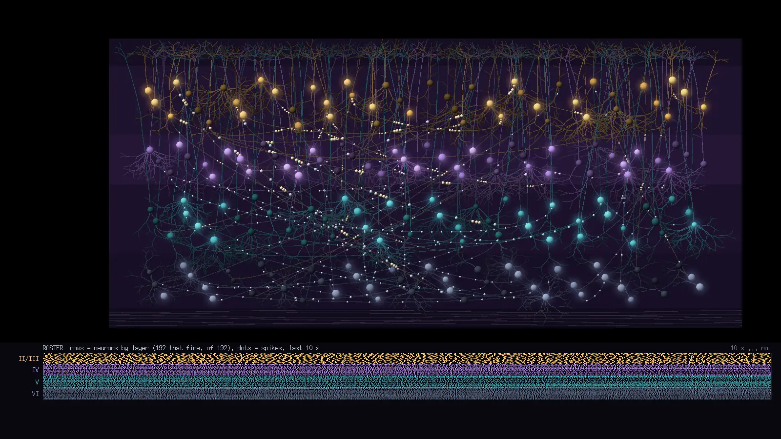
The README image of the view (docs/media/cortex.webp), rendered from the demo workload.

The system being modelled

The neocortex is a six-layered sheet of neurons that talk by action potentials, brief all-or-nothing voltage spikes of about a millisecond, conducted along axons and delivered across synapses after a delay. Neurons differ in how they turn a steady input current into a spike train: some fire regularly and slow down (regular spiking), some fire in bursts (chattering, intrinsically bursting), some fire fast without adapting (fast spiking). A recording rig shows this as a raster, rows being neurons and dots being spikes, and as membrane-potential traces.

The metaphor for a machine is direct. A process is a cell with an input drive (CPU), many short-lived sub-units (threads), and connections to other cells (sockets and pipes) that carry events. The loose point is that busy processes that talk synchronise, which is what coupled spiking neurons do and what request-handling services do under load. The honest limit: a neuron's spikes come from a model equation fed by CPU, not from anything the process does at spike times. They are a rendering of a smoothed CPU number through a nonlinearity.

History

The longer account lives in the repository: docs/theory/cortex.md.

The neuron. In the 1880s and 1890s Camillo Golgi's silver stain showed nerve cells in their entirety for the first time, and Santiago Ramon y Cajal used it to argue that the brain is made of separate cells that touch rather than a continuous net. Their opposed interpretations shared the 1906 Nobel Prize. Cajal's drawings of cortex, with its layers of pyramidal cells, are still reproduced. Korbinian Brodmann mapped the cortex into numbered areas in 1909.

The equations. Louis Lapicque (1907) modelled a neuron as a leaky capacitor that fires when it reaches a threshold, the integrate-and-fire model, which is crude and has survived a century because it is cheap. In 1952 Alan Hodgkin and Andrew Huxley worked out the ion currents in the giant axon of the squid and wrote them as four coupled equations, which won them a Nobel Prize in 1963 and remain the standard of biophysical realism. McCulloch and Pitts (1943) abstracted the neuron to a threshold logic gate, the root of artificial neural networks. FitzHugh and Nagumo (1961 to 1962) found a two-variable reduction of Hodgkin-Huxley that exposes its geometry.

The compromise. Eugene Izhikevich published his simple model in 2003. It is as cheap as integrate-and-fire (a few arithmetic operations per step) yet can be tuned to reproduce the firing patterns of many cell types, and it let him simulate tens of thousands of cortical neurons in real time on a desktop machine. Wolfgang Maass (1997) had called spiking networks the "third generation" of neural network models, the ones that compute with when a spike happens as well as how many.

The measure. David Golomb and John Rinzel (1993) proposed the synchrony index used here, in their study of networks of mutually inhibiting neurons.

Theory

The model is derived on Math Spiking Neurons; this section is what the view uses.

Izhikevich neurons

$$ \dot v = 0.04,v^{2} + 5v + 140 - u + I, \qquad \dot u = a,(b,v - u), \qquad v \ge 30\ \mathrm{mV} \Rightarrow v \leftarrow c,\ u \leftarrow u + d . $$

Here $v$ is the membrane potential in mV, $u$ a recovery variable, $I$ the input current, time is in milliseconds, $a$ is the recovery rate, $b$ its sensitivity to $v$, $c$ the post-spike reset potential and $d$ the post-spike jump in recovery. The quadratic is a fit to the shape of a real spike upstroke, not a derived quantity.

The rheobase

Set $\dot v = 0$ and $\dot u = 0$ with $u = bv$: the resting state satisfies $0.04v^{2} + (5-b)v + 140 + I = 0$. With $b = 0.2$ and $I = 0$ the roots are $-70$ mV (stable, the resting potential) and $-50$ mV (a saddle, the threshold). The discriminant $4.8^{2} - 0.16,(140 + I) = 0.64 - 0.16,I$ vanishes at $I = 4$, where the two collide and annihilate in a saddle-node bifurcation on an invariant circle. Below the rheobase, the smallest current that makes the neuron fire repeatedly, the cell rests; above it the rate rises from zero (Type I excitability). Because the reset lets a spiking cycle coexist with the resting state, the real onset sits a little under 4.

Four firing patterns

Code	Pattern	$(a, b, c, d)$	Kind drawn with it	Layer
FS	fast spiking	(0.1, 0.2, -65, 2)	kernel	VI
RS	regular spiking	(0.02, 0.2, -65, 8)	system	V
CH	chattering	(0.02, 0.2, -50, 2)	session	II/III
IB	intrinsically bursting	(0.02, 0.2, -55, 4)	container	IV

Fast-spiking cells are inhibitory interneurons that follow strong drive without adaptation; regular-spiking cells are the cortex's main excitatory cell, and a large $d$ makes them adapt; a high reset potential $c$ keeps chattering and bursting cells near threshold after a spike, so they fire in bursts. Pairing a pattern with a layer by process kind is a convention of the view: real neocortex has fast-spiking cells in every layer.

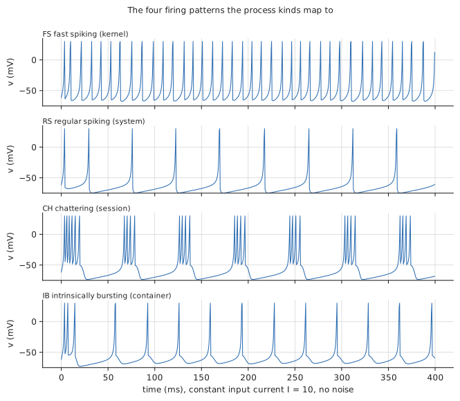
The four patterns at a constant current of 10 with no noise: one equation, four sets of $(a, b, c, d)$. From the repository's theory page.

From CPU to current

CPU runs from 0 to several hundred percent, while the neurons want a current in the range where the rate curve does something. A single linear map would give an FS and an RS cell very different rates for the same CPU, so neurons::calibration measures two currents per pattern once, without noise: the smallest that gives 1 spike/s (rheobase) and the one that gives 40 spikes/s (forty_hertz), each found by a scan in steps of 0.5 and then nine bisections (to about 0.001); a candidate current is settled for one second and its spikes counted over the next two. Replaying the update rule gives these noise-free currents (the repository's theory page):

Pattern	1 spike/s (rheobase)	40 spikes/s
FS	3.87	5.16
RS	3.78	19.0
CH	3.78	6.54
IB	3.78	12.3

An RS cell needs nearly four times the drive of an FS cell to fire at 40 Hz, because its large $d$ makes it adapt. neurons::current then interpolates piecewise linearly between landmarks of the share of one core $s = \mathrm{cpu}/100$:

$s$	0	0.005	0.05	1	3 and above
current	0	$0.62,r_h$	$0.98,r_h$	$I_{40}$	$I_{40} + 2,(I_{40} - 0.98,r_h)$

with $r_h$ the rheobase and $I_{40}$ the 40 Hz current. Idle is silent; half a percent is well below firing; five percent sits just short of the rheobase; one core fires near 40 Hz; and an active neuron (drive above 0) gets a Gaussian current noise of standard deviation 1.2 per step (NOISE), seeded from its identity, which keeps neurons with equal drive from firing in lockstep. Five percent of a core sits at $0.98,r_h$, at the edge of the onset, so the noise decides whether such a cell fires; the Python replay behind the calibration figure below, run with noise, gave 6 to 20 Hz at 5 % for the four types, not sporadic single spikes (a replay, not a measurement of the Rust view).

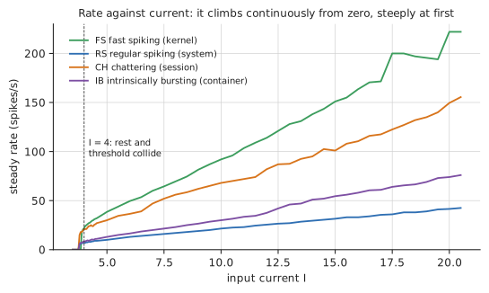
Steady rate against input current from a replay of neurons::advance; the onset sits just under $I = 4$ for all four types. From the repository's theory page.

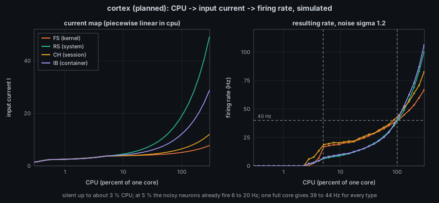
docs/figures/cortex-calibration.py, a Python replay with noise, 0.5 ms steps and 4 s windows after a 0.5 s settling, so its windows differ from the 1 s and 2 s of the Rust calibration; read the shapes, not the last digit.

Synapses and delay

When a neuron fires, a spike leaves along each of its axons and arrives after a conduction delay of at least one tick; on arrival the target takes a pulse of synaptic current $w$ that decays with a time constant of 5 ms:

$$ I_\mathrm{syn}(t + \Delta t) = I_\mathrm{syn}(t),e^{-\Delta t/\tau}, \qquad \tau = 5\ \mathrm{ms}. $$

The weight of a socket link of $B$ bytes per second is

$$ w = \min!\left(2,\ \tfrac14 \ln!\left(1 + \frac{B}{1000}\right)\right), $$

which gives $w = 0.25 \ln 2 = 0.17$ at 1 kB/s, 1.73 at 1 MB/s, and reaches the cap of 2 at $B = 1000,(e^{8} - 1)\ \mathrm{B/s} \approx 3$ MB/s: four decades of traffic spread over about one unit of weight. Where traffic is not measured the same log is taken of the socket count, $w = 0.25\ln(1+n)$ (0.35 for three sockets).

Synchrony

Golomb and Rinzel's measure asks how much of each neuron's variance over time is shared with the population mean:

$$ \chi = \sqrt{\frac{\mathrm{Var}_t\big(\langle V \rangle\big)}{\big\langle \mathrm{Var}_t(V_i) \big\rangle_i}} . $$

$\chi = 0$ for neurons that never agree and $\chi = 1$ for neurons that always do; for $N$ independent neurons it is about $1/\sqrt{N}$. Network::synchrony computes it from exponential running averages of $V$ and $V^{2}$ with a time constant of 2 s (VARIANCE_TAU), so it needs no stored history, and returns None (shown n/a) for fewer than two neurons or for neurons that hardly vary.

Mapping

Visual element	Measured quantity (source)	Transform
Soma	one process	pickable sphere; grows in on birth (Stage::growth); radius $0.45 + 0.35\min(\sqrt{\mathrm{GiB}}, 2)$ world units from Process.memory (soma_radius: 0.45 for a tiny process, 0.80 at 1 GiB, 1.15 from 4 GiB)
Layer	Process.kind	bands of the 56-unit slice height: I molecular 10 % (empty), II/III session 25 %, IV container 18 %, V system 25 %, VI kernel 20 %, white matter 7 %, scaled by their sum 1.05
Seat in the layer	lifetime seat per layer (layout::Seats)	point $n$ of the R2 sequence, $({0.7549,n}, {0.5698,n})$, in the band's middle 72 %, plus a seeded jitter; stable for the life of the process
Firing pattern	Process.kind	the table above (Firing::of)
Input current	Process.cpu (the collector's smoothed figure)	neurons::current, the piecewise map above
Primary dendrites	Process.threads	one per thread, clamped to 1 to 12 (MAX_PRIMARIES); each grows from its own seed and forks twice, so a count of 500 draws 12 and a count of 0 draws 1; decorative in shape
Apical dendrite (layered cells only)	none	trunk up to layer I with a tuft; carries no data
Axon	a socket link in Snapshot.links, or a pipe or FIFO in Snapshot.pipes	one cubic arc below the two somas for each linked pair (24 segments, a little different for every pair), a synapse for each direction a spike may take: both for a socket, writer to reader for a pipe (both for a two-way pipe)
Synaptic weight	Snapshot.link_traffic (loopback TCP bytes per second)	$\min(2, \tfrac14\ln(1 + B/1000))$; the socket-count form when traffic is unmeasured; a pipe has the fixed PIPE_WEIGHT 1.0, because neither platform measures pipe throughput
Conduction delay	the arc's length in world units	CONDUCTION = 125 units/s (the unwidened 100-unit slice in 0.8 s), rounded to whole 0.5 ms ticks, at least one
Pulse on an axon	an in-flight spike event of the network	ball of $1.7 + 0.8w$ px along the arc; at most 3,000 drawn (every $n$th in flight when there are more)
Soma flash	a spike	brightness and glow decaying as $e^{-t/0.06,\mathrm{s}}$ over the last 0.3 s (FLASH_TAU)
Soma brightness	firing rate over the last second, and depth	$0.34 + 0.25,\mathrm{depth} + 0.25\min(\mathrm{rate}/40, 1)$ plus the flash
Raster dots	spike ticks of the last 10 s	the bottom 22 % of the frame; a row for each neuron that fired, ordered by layer then seat, binned when rows would be under 2 px; three brightness levels by spikes per cell
$\chi$ in the legend	membrane potentials of the talking neurons	neurons with a link and at least 5 % CPU (TALKING_CPU), averages with 2 s time constant
Sparkline in the inspector	the selected neuron's $v$	the last 320 ms (640 ticks), -80 to +30 mV, 40 braille cells in two rows
Dust of an exit	a process that left	the soma shrinks over 1.2 s and 12 seeded specks fly off (DUST_SECONDS, DUST_SPECKS)
Layer fill, white-matter fibres, dendrite and axon shapes	none	decorative

How isotop realises it

Module and row. src/neurons.rs is the simulation with no drawing; src/cortex.rs holds Cortex (layout, axons, drawing, raster) implementing views::ViewModule. The registry row sets links: LinkRule::DrawnByView (axons follow the c link key, which Stage::links carries), link_strokes: true, haze: false (the slice is a drawing, not a scene to haze), pitch and face to the isometric pitch (the slice is an upright plane facing the default camera), sources: Sources::of(&[Source::Pipes]), Backdrop::Void, demo option channels: true (synthetic Unix-socket queues and pipes), and a warm-up that plays 12 s of demo at a 0.1 s step so the raster is full at 12 s. No view-local keys and no digit.

Clock. simulation::FixedStep with the 0.5 ms tick (neurons::STEP_SECONDS) and a catch-up of CATCH_UP = 0.1 s per frame, that is at most 200 steps; a longer gap is dropped, so a pause freezes the simulation. Neurons run in real time: a 40 Hz neuron fires every 25 ms of wall clock. Everything counts in whole ticks, so two runs that take the same steps give the same spikes, whatever frame rate asked for them.

Integration. neurons::advance takes one explicit Euler step of 0.5 ms, clamps $v$ at 30 mV, and applies the reset when it sees $v \ge 30$ at the start of the next step.

Event queue. A spike in flight is a small tuple of arrival tick, synapse index and emission tick in a binary heap ordered by arrival; each step pops what is due, adds the weights to the targets' synaptic current, and fires whichever neurons crossed 30 mV. The queue holds at most MAX_EVENTS = 262,144 spikes; one beyond is lost, as a saturated machine would lose one. At 2,000 ticks per second a 20 ms delay is 40 ticks.

Layout. A process keeps its seat in its layer for life. When a layer outgrows the slice's capacity (one neuron per $2.2 \times 2.2$ units of 72 % of the band) the slice widens by 1.25 (WIDENING) and never narrows again, so a seat never changes but positions scale with the width. Exits never shrink it.

Drawing. Dendrites, axons and the white-matter fibres are hairlines at depth biases that stack strokes behind pulses behind somas; somas are lit spheres; flashes are Item::Glow; the raster panel is screen-space whole-pixel triangles and Item::Glyph lettering in front of the slice, so the CPU and GPU rasterizers agree on it. Above 400 neurons (CROWD), or when a soma is under 3 px, only primary dendrites are drawn.

Rewiring. Axons and synapses are rebuilt when the sample or the set of neurons changes (Cortex::rewire); the selection's connected component, for its own $\chi$, is found again when they are.

Inspector and tour. The selected neuron's lines are: type and $(a, b, c, d)$, I and rate over 2 s, layer and threads drawn of total, synapses in with the minimum and maximum delay in ms, the component's $\chi$ and neuron count, and the braille trace. The tour's callout for each of the 16 busiest processes reads FS 40 Hz | I 5.2 | layer VI in that form.

Legend. chi 0.18 talking | 594 spikes/s | ... (n/a while $\chi$ is unknown), then the status::missing_note wording for Source::SocketTraffic ("weight = socket count") and Source::Pipes ("pipes are not drawn") while they apply, then | soma = process, layer by kind | dendrite = thread | axon = link, delay ~ length, weight ~ log traffic | current ~ CPU. The numbers shown here are an example of the format, not a captured legend.

Platforms. Linux: full. Where the platform cannot read per-link traffic the weight is the socket-count form and the legend says so; I did not confirm on macOS which source reports as missing (unverified). Pipes are scanned on both platforms.

Reading the picture

• Measured: which processes exist, their kind (the layer), their smoothed CPU (through the current map), thread counts (the dendrites), memory (soma radius) and which processes share a socket or pipe (the axons). Traffic gives the synaptic weight of a socket.
• Derived: the spikes. They are a deterministic function of the smoothed CPU, seeded noise and incoming spikes. A spike does not mean the process did something now; it means the model neuron crossed its threshold. Two processes at the same CPU fire at different times because of their noise seeds.
• Real in order, decorative in speed: a pulse is a spike event that was generated, queued with its delay and arrives; the 0.8 s slice crossing is a display choice, roughly two orders of magnitude slower than cortical conduction.
• Resolution. The raster is about one frame wide for 10 s, so one pixel is several milliseconds at 1080p: a burst with 2.5 to 4.5 ms intervals is one cell and a 100 Hz neuron a solid bar. A 40 Hz neuron (25 ms period) flashes steadily rather than visibly pulsing, since the flash lasts 60 ms; spikes above about 30 Hz cannot be resolved by eye.
• Cannot infer: CPU from the firing rate (the four patterns give different rates for the same CPU), causal influence between processes (an axon says only who is connected, and socket synapses are excitatory both ways), or any real neuroscience.
• Aliasing. The membrane state is simulated at 2 kHz and sampled by the frame loop for drawing; the sparkline reads the state, not frames.

Try it

Run here with the release binary (Linux, CPU renderer):

./target/release/isotop --demo --view cortex --time 12 --width 1600 --output /tmp/cortex.png --renderer cpu

Output: Wrote /tmp/cortex.png (1600x900, 192 visible). Live: ./target/release/isotop --view cortex, or Tab and the v picker (cortex is the fifteenth row of the registry, so it has no digit). c cycles the link mode: with links off no axon or pulse is drawn, though the simulation runs on. Click a soma to read its inspector and its membrane sparkline. Not run here: a live (non-demo) session.

Where in the code

Item	Path and symbol
Simulation	src/neurons.rs: Firing, advance, calibration, current, Network (step, synchrony, in_flight), sparkline
View	src/cortex.rs: Cortex, LAYERS, Slice, Body, Axon, weight_of_rate, weight_of_sockets, soma_radius, raster_bins, Cortex::rewire
Registry row	src/views.rs: REGISTRY row cortex
Shared helpers	layout::Seats, simulation::FixedStep, Rng::for_identity, glyphs, terminal::clean_sparkline
Links	Snapshot.links, Snapshot.link_traffic, Snapshot.pipes in src/model.rs
Repository theory page	docs/theory/cortex.md
Prototype (reference only)	docs/mockups/code/cortex.py

Variations and open questions

• The roadmap specified the raster and the dendrites as beams and the pulses as glows; the implementation draws the raster as whole-pixel triangles with bitmap lettering, the dendrites and axons as hairlines, and the pulses as small spheres. It also uses memory, which the roadmap left unused, for the soma radius, and pipes, which the roadmap did not yet have, for axons with a fixed weight.
• Add an inhibitory population (kernel threads as fast-spiking interneurons with negative weights, their biological role) and see whether $\chi$ discriminates better.
• Compare $\chi$ of a connected component against shuffled links as a null model.
• Let Process.priority set the resting potential.
• Replace the fixed PIPE_WEIGHT by a measured throughput, where either platform can measure one.
• Layer I is declared empty in LAYERS (kind: None) and is nearly empty in the animal. Lower NOISE from 1.2 to 1.19 and see whether the demo's $\chi$ at 12 s changes in the second decimal (untried).
• One OOM kill is drawn four ways in this program: a plunge in View Horizon, a stone in View Necropolis, a fox in View Coop, a puff of dust here. No two of them agree on how long the dead should be looked at.

References

• E. M. Izhikevich, "Simple model of spiking neurons", IEEE Transactions on Neural Networks 14 (2003) 1569-1572; "Which model to use for cortical spiking neurons?", IEEE Transactions on Neural Networks 15 (2004) 1063-1070; Dynamical Systems in Neuroscience, MIT Press (2007).
• D. Golomb and J. Rinzel, "Dynamics of globally coupled inhibitory neurons with heterogeneity", Physical Review E 48 (1993) 4810.
• A. L. Hodgkin and A. F. Huxley, Journal of Physiology 117 (1952) 500.
• W. Maass, "Networks of spiking neurons: the third generation of neural network models", Neural Networks 10 (1997) 1659-1671 (unverified volume and pages).
• See also Math Spiking Neurons, Theory Simulation Toolkit, Theory Text Safety.