View Strata

View: Strata

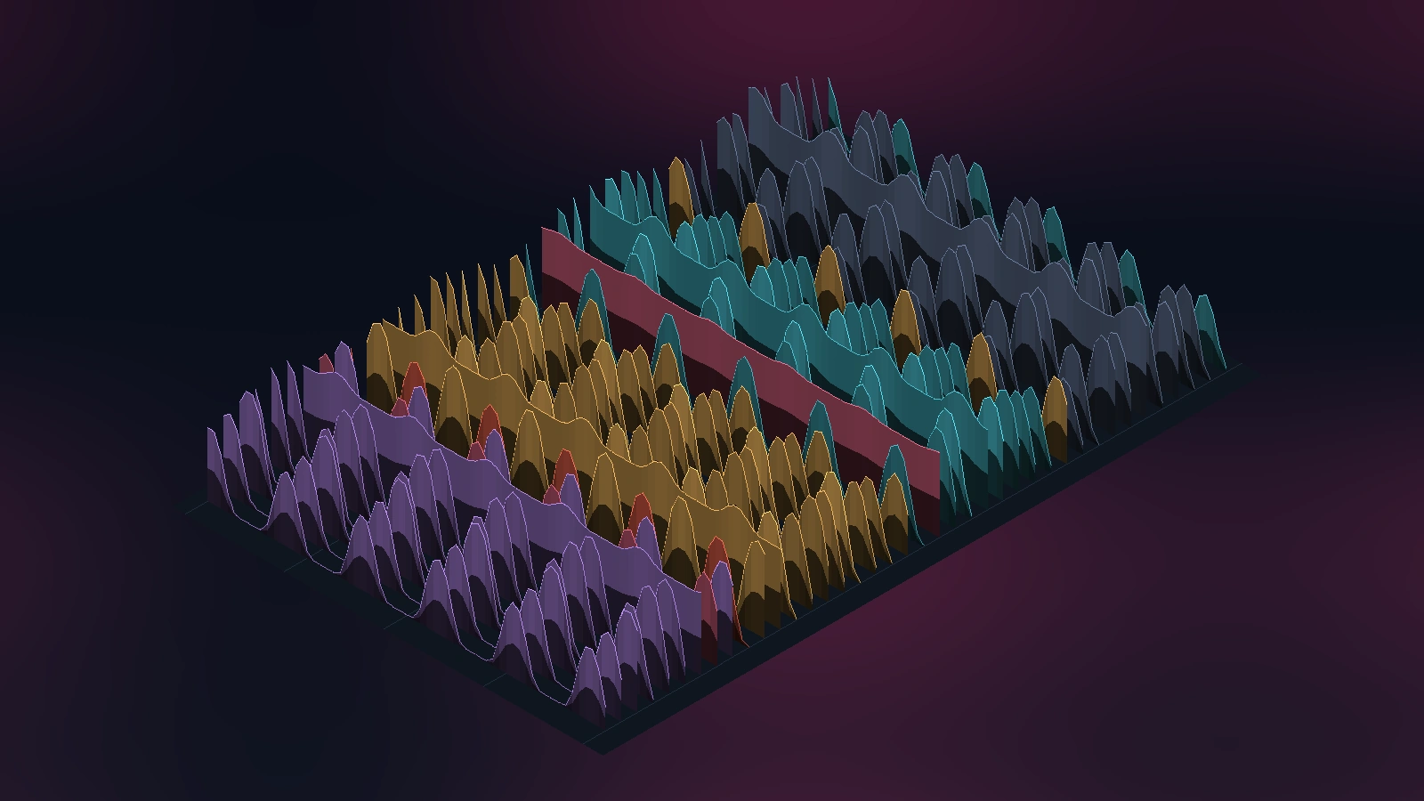
Strata is the last minute of CPU use as a ridgeline landscape. Each of up to forty busy processes is a ridge whose height traces its CPU use over time, with now at the front edge; rows run from kernel threads at the back through system services and your session to containers at the front, and a ridge keeps its row for as long as it stays busy. Nearer ridges are opaque walls, so what is behind them is hidden, as on the cover of a famous record sleeve. The history is recorded in every view, so the landscape is already a minute deep when you switch to it.

The system being modelled

The ridgeline form

A ridgeline (or joy plot, or waterfall plot in vibration analysis and radio astronomy) stacks many 1-D signals one above another with a small vertical offset, each drawn as a line, and hides the parts of a line that a nearer one covers. It is the standard way to show how one profile changes over a second dimension: a spectrum over time, a pulse shape over successive pulses, a distribution over categories.

The best-known instance is the sleeve of Joy Division's Unknown Pleasures (1979), designed by Peter Saville. The stacked white lines on black are, as widely reported, a plot of successive radio pulses from the pulsar CP 1919 (PSR B1919+21), the first pulsar found, discovered by Jocelyn Bell (later Bell Burnell) and Antony Hewish in 1967 and announced in Nature in 1968. The plot itself is generally credited to Harold Craft's 1970 Cornell thesis on pulse profiles, reproduced in the Cambridge Encyclopaedia of Astronomy (1977), from which Saville took it and inverted it to white on black. (The thesis is Harold D. Craft Jr., "Radio Observations of the Pulse Profiles and Dispersion Measures of Twelve Pulsars", Cornell, September 1970; the route through the 1977 Cambridge Encyclopaedia of Astronomy is as Scientific American's account of the sleeve's origin gives it.) The relevance to isotop is the construction, not the astronomy: in the pulsar plot each row is one pulse at successive times with the horizontal axis the phase within the pulse period; in Strata each row is a different process with the horizontal axis time. A pulsar's pulses repeat; processes do not.

Hidden-line removal

Showing only what is visible is the hidden-surface problem. Three classical solutions matter here.

• Painter's algorithm (Newell, Newell and Sancha, 1972): sort the objects far to near and paint each over what is already there. For a ridgeline it is the whole algorithm: draw the farthest row first, fill under its line with the background colour, draw the next row over it.
• Depth (z) buffer (Catmull, 1974): keep, per pixel, the depth of the nearest thing drawn so far and overwrite only when a new fragment is nearer. Order does not matter.
• Floating horizon: a method specific to height fields that tracks, per screen column, the highest line drawn so far and draws only what rises above it.

History

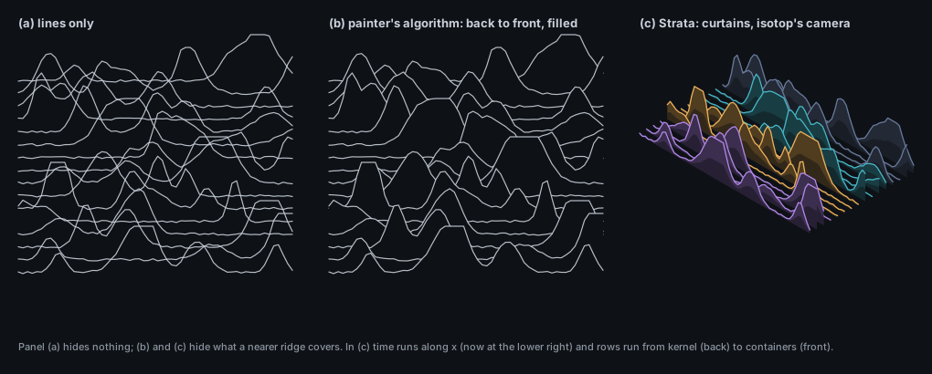
The thing Strata draws is the stacked-profile plot, and the long argument about how to hide the lines that lie behind other lines.

• Pulsar CP 1919 was found by Jocelyn Bell and Antony Hewish in 1967 and announced in Nature in 1968 (see the section above). Craft's 1970 thesis plotted its successive pulses one above another; Scientific American's account puts the number at 80 consecutive pulses at 318 MHz. A few months later the plot appeared in Scientific American as white lines on cyan, in 1971, before the 1977 encyclopaedia and Saville's inversion to white on black. Strata stops at forty ridges, half of that.
• The same construction is known by other names in other fields: the waterfall plot of vibration analysis and radio astronomy, and in statistics the ridgeline plot. The statistics community called it the joyplot for a few months: the name was proposed by Jenny Bryan in a tweet of 24 April 2017, and Claus Wilke renamed his package ggjoy as ggridges in September 2017 after learning where the band took its own name from.
• Making such a plot readable is the hidden-line problem. Newell, Newell and Sancha described the painter's algorithm in 1972, and Catmull described the depth buffer in his 1974 thesis at Utah. Strata uses the second because the hardware does, and the first would give the same picture.
• A third classical answer, the floating horizon, belongs to height fields specifically and is described above; its history is not given here.
• The relevant detail for Strata is that the thing plotted has changed meaning along the way. The pulsar plot has pulses on one axis and phase on the other, and a pulsar repeats; the strata of this page have time on one axis and processes on the other, and processes do not.

Theory

From a counter to a profile

Each point of a ridge is a sampled value of a filtered rate. The kernel counts a process's CPU time, a cumulative counter; isotop differences it over the sampling interval $\Delta t$ (a boxcar average of the instantaneous use), then smooths the result with a one-pole filter of time constant $\tau = 1.5$ s,

$$ c_k = c_{k-1} + \bigl(1 - e^{-\Delta t/\tau}\bigr),(r_k - c_{k-1}), $$

with $r_k$ the interval's raw use in percent of one core. The history stores $c_k$ (Process::cpu), not $r_k$. Consequences:

• A step to 100 % reads 49, 74, 87, 93 ... percent over the next samples at $\Delta t = 1$ s, and a single second at 100 % reads 49, 25, 13, 7 ... : the area under the ridge is conserved (it is the CPU time), but its edges are smeared forward in time by about $\tau$.
• The filter has its half-power point at $f = 1/(2\pi\tau) \approx 0.106$ Hz, a period of 9.4 s. Faster wiggles are attenuated; wiggles faster than twice the sampling rate are aliased before the filter can touch them, because the boxcar average over $\Delta t$ is a poor anti-alias filter. A ridge is a low-pass picture of the process's CPU use.

Height

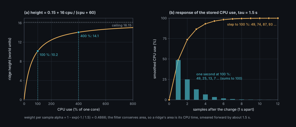
Raw CPU percent is unbounded (a process with 32 threads can use 3200 %), and a ridge must fit in a row. Strata uses the saturating map

$$ h(c) = 0.15 + 16,\frac{c}{c + 60}, $$

which is 10.2 world units at 100 % (one whole core), 14.1 at 400 % and approaches 16.15. A process that is absent from a sample in the window is drawn at the floor, $h(0) = 0.15$.

The time axis

A sample taken at elapsed seconds sits at ground coordinate $x = (\text{elapsed} - \text{now} - \text{scroll})\cdot 1$, one unit per second, so the window of 60 s spans $x\in[-60, 0]$ and the tick labels read now, -15 s, -30 s, -45 s, -60 s. now is the shown snapshot's elapsed, so pausing or rewinding shows the minute that ended there. While the shown snapshot is the newest, scroll runs from 0 to the sampling interval since the newest sample arrived and the last value is held out to $x = 0$: the landscape slides at constant speed between samples instead of stepping once a second. In a paused or rewound view the scroll is 0.

How much history exists

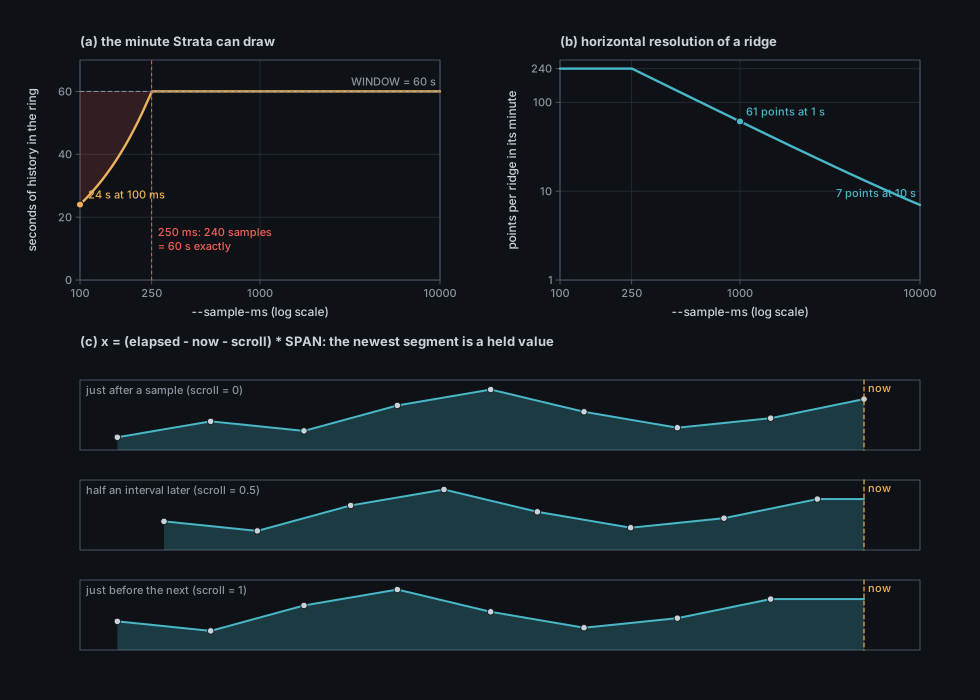
The shared history (src/history.rs, see Theory: History) is a ring of CAPACITY = 240 samples, and Strata asks for a time window of 60 s by Sample::elapsed. At the default --sample-ms 1000 the ring holds four minutes and the window is full. The number of seconds the ring can answer with is $\min(60, 0.240,\Delta t_{\text{ms}})$; the minute is complete only for --sample-ms of 250 or more, and at --sample-ms 100 Strata's "minute" is 24 s (issue #127: retention should be sized by time, not by sample count). At the other end, a long interval leaves few points: --sample-ms 10000 gives a ridge of seven points.

Mapping

Visual element	Measured quantity (platform source)	Transform
Ridge	A process whose CPU reached 0.5 % at some sample in the last 60 s	At most 40 ridges; BUSY = 0.5
Ridge height at a sample	Process::cpu in that sample (model-smoothed percent of one core): /proc/<pid>/stat utime and stime, macOS proc_pid_rusage	$0.15 + 16,c/(c+60)$
Position along the ridge	The sample's elapsed (seconds since the run began)	$x = $ elapsed $-$ now $-$ scroll, 1 unit per second, window 60 s
Row	Process kind, then free rows by heat	40 rows; kernel (rows 0 to 9), system (10 to 19), session (20 to 29), containers (30 to 39) back to front; a newcomer takes the free row nearest the middle of its quarter; spacing 2.4
Ridge colour	Kind (kind_color) with state override (zombie, stopped, blocked)	The current colour of the process, applied to the whole ridge
Wall shading	Local height	Lower 45 % tint $0.10 + 0.12f$, upper $0.20 + 0.45f$, ridge line $0.75 + 0.6f$, with $f = (z_0 + z_1)/(2\cdot 16)$
Row label	Process name and current Process::cpu	label_name (at most 15 cells), at $x = 1.5$
Inspector note	History window	peak P% CPU over the last S s, with $S$ the span actually covered
Floor, 15 s ticks, now	none	Decorative scale; the ticks are exact

How isotop realises it

Recording. Strata is a ViewModule in src/strata.rs: the state struct Strata holds only the row assignments, and its registry row in views::REGISTRY builds it with a closure. Scene::record records the history on every sample whichever view is shown, so Strata reads stage.history and needs no record of its own. In --demo --output runs the row's warm-up (Phase::History { seconds: 60 } under When::DemoOutput) replays a minute of demo samples; a live headless run takes two samples to measure CPU, so live Strata then shows only its newest slice.

Row assignment. Strata keeps rows: HashMap<Identity, usize>. A ridge keeps its row while its peak over the window stays at least BUSY; otherwise the row is freed. Rows are offered to every sampled process, drawn or not, drawn first and then by descending peak, ties by Identity, so focus and --limit free none of them: clearing them brings each ridge back to its row. When all 40 rows are taken a drawn process takes the row of the least busy hidden holder. A newcomer's row is the free one nearest rank * 10 + 5 for its kind's rank, spilling into neighbours when its quarter is full; a ridge never moves between rows during its life.

Geometry. Each ridge is a vertical curtain in the plane $y = 2.4\cdot\text{row}$. For each pair of consecutive profile points Strata::draw (the ViewModule::draw implementation) emits two quads, the lower band from the floor to 45 % of the height and the upper from there to the profile, and a line along the profile; the last point is repeated at $x = 0$ (the held value) and a ridge with a single sample point gets a leading point one interval earlier. Quads carry the process's pick index; lines leave nothing pickable. The camera is the usual orthographic isometric one, so a curtain's front face shows.

Hiding. The display list is depth-tested by both rasterizers (CPU Frame::rasterize and the wgpu shader), so the nearer curtains hide the farther without any sorting by the view: the painter's order of the figure above gives the same picture because each curtain is planar, but the implementation is the z-buffer. See Theory: Rasterization and Theory: Scene and display list.

Camera and bounds. The fit uses a fixed envelope, the floor plus a height of $0.7\times 16$, so it does not jump as ridges rise. The front of each ridge, $(0, y, \text{top})$, is its pick anchor and stage.positions entry.

Time step. Strata has no simulation and does not use stage.dt; its only time dependence is scroll, derived from stage.time and the time the history's newest sample arrived.

Stable layout. Rows are stable by construction and the harness enforces it (the row waives nothing). The profile of a ridge changes only by new samples arriving at the front.

Sources. CPU only (Process::cpu). No optional source is demanded, so nothing here appears in Snapshot::missing.

Reading the picture

• Height is smoothed CPU, not instantaneous. Peaks are lower and later than the raw bursts that made them; a ridge's area is its CPU time.
• Heights saturate. Above about 400 % the curve is flat to the eye; a process on 1600 % and one on 400 % differ by 1.5 world units. Do not compare tall ridges.
• Absent is zero. A process that did not exist for part of the minute is drawn at the floor there; the picture does not mark births. A process that exits vanishes from the landscape at its next sample and its row is freed.
• Rows are ranks, not rankings. A ridge's row does not say which process used more; the kind owns the quarter.
• Colour is current. A ridge turns pink or orange for its whole length if the process is a zombie or stopped now.
• Hidden is hidden. Tall ridges at the front hide low ridges behind them; click or use search to find a covered one. The 40-ridge cap hides the rest, and the legend's collapsed count counts them.
• A short history is shown as short. Only the samples the ring holds are drawn; the left end of the floor is empty.
• The window depends on --sample-ms. See issue #127.

Try it

./target/release/isotop --demo --view strata --output strata.png --width 1600 --renderer cpu
./target/release/isotop --demo --view strata --time 90 --output strata90.png
./target/release/isotop --view strata --sample-ms 100     # live: the minute is truncated to 24 s

Press 7 in a session. The demo's CPU is $\tfrac{\text{scale}}{16}(1+\sin\theta)^4 + \text{bonus}$ with $\theta = 0.55,t + 1.71,i$ for process $i$: narrow peaks every $2\pi/0.55 = 11.4$ s with long troughs, phase-shifted per process, which is why the demo ridges show five or six peaks across the minute. Headless PNGs carry no row labels, which are terminal overlays.

Where in the code

• src/strata.rs: Strata, Strata::draw, Strata::legend; constants WINDOW, ROWS, SPAN, SPACING, PEAK, BUSY.
• src/history.rs: History::record, window, newest, arrived; CAPACITY, SERIES.
• src/model.rs: measure (the 1.5 s smoothing), bounded, demo_cpu_integral and the demo CPU shape.
• src/views.rs: the strata row (Phase::History { seconds: 60 } under When::DemoOutput); the legend is Strata::legend.
• src/palette.rs: kind_color.
• Figures: docs/figures/strata-ridgeline.py, strata-window.py, strata-response.py.

Variations and open questions

• Retention by time (issue #127): size the ring by the longest window any view reads.
• Raw and smoothed side by side. History stores the model's smoothed CPU; storing the interval's raw rate would let a ridge show the boxcar average (sharper edges) and a second line the smoothed one.
• Colour a ridge by its own history. Use the kind at each sample, so a zombie's ridge turns pink only where it was a zombie.
• A ridge per cgroup. Sum a cell's members and compare with Cells.
• Spectral Strata. Replace the time axis by frequency and the rows by windows of time (a waterfall plot of the CPU spectrum), which would make periodic processes line up as vertical streaks.
• Open: is the saturating knee at 60 % the right one? A log height would separate 1 %, 10 % and 100 % ridges that now share the floor.

References

• P. Saville, sleeve of Joy Division, Unknown Pleasures (Factory Records, 1979).
• A. Hewish, S. J. Bell, J. D. H. Pilkington, P. F. Scott, R. A. Collins, "Observation of a rapidly pulsating radio source", Nature 217, 1968, pp. 709-713.
• M. E. Newell, R. G. Newell, T. L. Sancha, "A solution to the hidden surface problem", Proceedings of the ACM Annual Conference, 1972.
• E. Catmull, "A subdivision algorithm for computer display of curved surfaces", PhD thesis, University of Utah, 1974 (the z-buffer).
• Related pages: Theory: History, Theory: Model and rates, Theory: Rasterization, Theory: Camera and projection, View: Ptolemy (which also reads a minute of history).