View Globe

View: Globe

Globe shows where the machine's TCP connections go. A sphere with Natural Earth coastlines turns once every five minutes; from home, a great-circle arc rises to every remote place a connection lands, brighter with more traffic, cyan when the place is mostly sending to this machine and pink when mostly receiving from it, with pulses travelling the way the bytes flow. The processes that hold the connections hover in a golden-angle cloud above home, and their inspector lists each connection with its round-trip time and byte rates, which come from the kernel's own tcp_info. Addresses with no known place circle the north pole, with a label that says why. Every lookup is local; nothing is sent anywhere.

The system being modelled

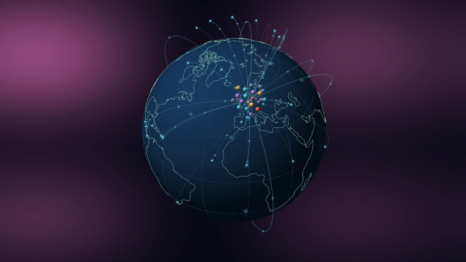
Three separate pieces of physics and geodesy meet in this view, and each is exact in the theory and approximate in the picture.

The sphere, seen without perspective. Drawing a globe on a flat screen is a map projection. The camera of isotop is orthographic: projectors are parallel, so a sphere of radius $R$ is always the disc of radius $R$ times a fixed scale, whatever its distance, and exactly one hemisphere is visible, bounded by the limb. This is the orthographic projection of cartography, the view of the earth from infinitely far away.

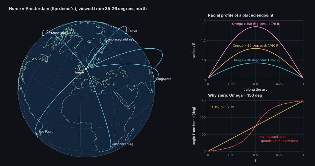
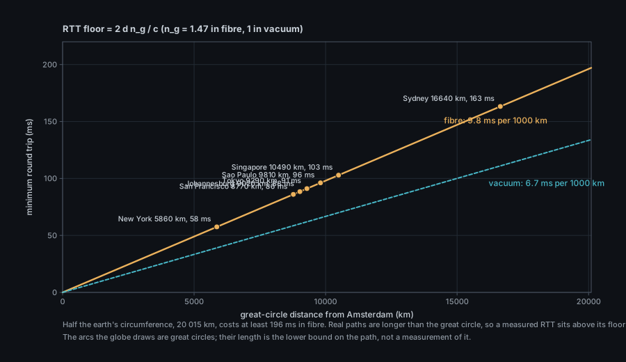
Great circles. The shortest path between two points on a sphere lies on the great circle through them, the intersection of the sphere with the plane through the two points and the centre. The arcs of the globe are great-circle segments. Network traffic does not follow them: it follows cables and routers. The arc is the geodesic lower bound on the path, not the path.

Where an address is. An IP address has no coordinates. A geolocation database maps address blocks to places by combining registry records, routing data and measurements, so a location is a statistical claim about a block: at best the city of the block's users, at worst the country's centroid, and wrong for anycast, content networks, mobile carriers and VPNs. isotop reports such a place as what the database says and never as a measurement.

History

The projection. The view of a sphere from infinitely far away, the orthographic projection, is among the oldest in the record. Hipparchus is credited with using it in the second century BCE to work out where stars rise and set, and for a long time it went by the name analemma. Its present name is generally credited to the Antwerp Jesuit Francois d'Aguilon, in his Opticorum libri sex (1613), the book Rubens illustrated; sources differ over whether he coined the word or took it from Vitruvius, and one older source applies the same coinage to the stereographic projection, so the attribution is not settled here. Mercator's cylindrical projection (1569) came 1,700 years later and answered a different question, how to draw a constant bearing as a straight line.

The meridian. A globe needs a zero of longitude, and for most of history there was none. The International Meridian Conference in Washington in 1884 chose Greenwich: 22 delegations voted for, San Domingo against, and France and Brazil abstained. It matters here because geo::home can fall back to longitude 0.

Coastlines. Computer cartography began with the geographic information systems of the 1960s, of which Roger Tomlinson's Canada Geographic Information System is the usual first example (the dates of its stages are unverified here). The coastlines in src/coastline.bin come from Natural Earth, a public-domain dataset published at scales of 1:10, 1:50 and 1:110 million by Tom Patterson and Nathaniel Vaughn Kelso, later maintained as a volunteer project supported by the North American Cartographic Information Society. isotop uses the coarsest scale. The launch year is not confirmed here.

Addresses to places. An IP address has no position. MaxMind, founded in 2002, says it coined the term GeoIP that year and launched a commercial address-to-location database; it later released a free subset, GeoLite. The legacy GeoLite files (GeoIP.dat) were retired on 2 January 2019 in favour of GeoLite2, in the MaxMind DB format; DB-IP publishes a compatible free city database. isotop reads both formats: see "Databases" below.

Theory

Orthographic projection, derived

Let the view be centred on latitude $\varphi_0$ and longitude $\lambda_0$ (the point of the earth directly facing the viewer). A surface point with latitude $\varphi$ and longitude $\lambda$ has the unit normal $n = (\cos\varphi\cos\lambda,\ \cos\varphi\sin\lambda,\ \sin\varphi)$ in an earth-fixed frame. The unit vector to the viewer is $v = (\cos\varphi_0\cos\lambda_0,\ \cos\varphi_0\sin\lambda_0,\ \sin\varphi_0)$. Choose screen axes at right angles to $v$: east, $e = (-\sin\lambda_0,\ \cos\lambda_0,\ 0)$, and "up", $u = (-\sin\varphi_0\cos\lambda_0,
-\sin\varphi_0\sin\lambda_0,\ \cos\varphi_0)$. The screen coordinates and the depth of the point are the three dot products:

$$ \begin{aligned} x &= n\cdot e = \cos\varphi,\sin(\lambda-\lambda_0),\\ y &= n\cdot u = \cos\varphi_0\sin\varphi - \sin\varphi_0\cos\varphi\cos(\lambda-\lambda_0),\\ w &= n\cdot v = \sin\varphi_0\sin\varphi + \cos\varphi_0\cos\varphi\cos(\lambda-\lambda_0). \end{aligned} $$

The point is on the visible hemisphere iff $w \ge 0$, and $x^2 + y^2 + w^2 = 1$ puts the limb ($w=0$) on the unit circle. A point at height $\rho R$ above the centre ($\rho > 1$) is hidden by the earth iff $w < 0$ and $x^2 + y^2 < 1$ (it lies behind the centre plane and inside the silhouette cylinder). Distances on the screen are true only at the centre: the radial scale factor is $\cos c = w$ and falls to zero at the limb, which is why coastlines crowd there.

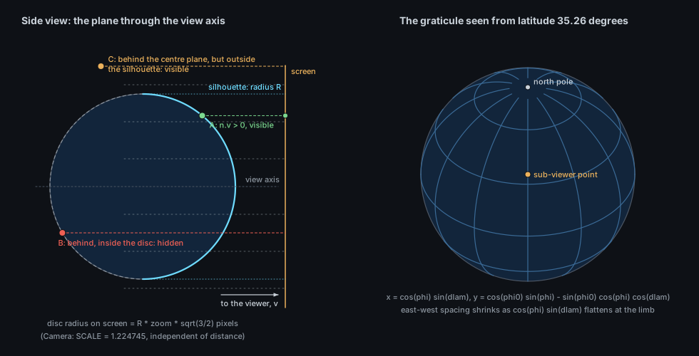
isotop's camera is this projection. Camera::view maps a ground point $(x,y)$ and height $z$, with rotation $\kappa$ and pitch $p$, to across = x cos(κ+π/4) - y sin(κ+π/4), along = x sin(κ+π/4) + y cos(κ+π/4), screen right $= \text{across}\cdot S$, screen up $= (z\cos p - \text{along}\sin p),S$ and depth $= \text{along}\cos p + z\sin p$, with $S = \sqrt{3/2} = 1.224745$ pixels per world unit at zoom 1. The globe places longitude $\lambda$ at azimuth $\theta = \text{spin} - \lambda$ with $\text{spin} = \pi/4 + \lambda_h + \dots$ ($\lambda_h$ the longitude of home). For rotation 0 the factor $\pi/4$ cancels: $\text{across} = R\cos\varphi\cos(\theta+\pi/4)$, which is $R\cos\varphi\sin(\lambda - \lambda_h)$, and $\text{along} = R\cos\varphi\cos(\lambda-\lambda_h)$. Substituting gives exactly the three equations above with $\lambda_0 = \lambda_h$ and $\varphi_0 = p$: the latitude at the centre of the disc is the camera pitch, 35.26 degrees at the default. Scrolling vertically adds a lean $\ell$ that rotates the whole earth about the screen-horizontal axis, moving the centre latitude to $p - \ell$ (clamped so it stays between the poles).

Rotation and tilt

The earth turns once in SPIN_SECONDS = 300 s, eastward: $\text{drift}(t) = -2\pi t/300$ radians of azimuth, and east is the direction of falling azimuth, which the camera draws on the right. A sidereal day is 86 164 s, so the turn is about 287 times faster than the real one. At time 0 home faces the default camera. There is no axial tilt of 23.4 degrees and no seasons: the earth's axis stands vertical in the scene and the "tilt" is whatever the viewer leans it to by scrolling (globe_tilt). A horizontal scroll turns it by hand (globe_turn) and holds it still until r or the tour lets it spin again.

Great circles: slerp and the haversine

Let $a$ and $b$ be the unit vectors of home and of the endpoint, and $\Omega = \arccos(a\cdot b)$ the central angle between them. The point at fraction $t$ along the great-circle arc lies in $\operatorname{span}{a, b}$, has unit length and is $t\Omega$ from $a$. Writing $p = \alpha a + \beta b$ and requiring $p\cdot a = \cos t\Omega$ and $p\cdot b = \cos(1-t)\Omega$ gives the linear system $\alpha + \beta\cos\Omega = \cos t\Omega$, $\alpha\cos\Omega + \beta = \cos(1-t)\Omega$. Using $\cos t\Omega = \cos\Omega\cos(1-t)\Omega + \sin\Omega\sin(1-t)\Omega$,

$$ \alpha = \frac{\sin\bigl((1-t)\Omega\bigr)}{\sin\Omega},\qquad \beta = \frac{\sin,t\Omega}{\sin\Omega}, $$

which is spherical linear interpolation (slerp; Shoemake, 1985) and sweeps the angle at a constant rate. The cheaper "interpolate linearly and normalise" does not: the chord's midpoint is nearer the centre, so the normalised point moves fastest in the middle (the dashed curve in the figure below, at $\Omega = 150^\circ$). The code uses the dot product, acos(clamp(dot)); for the central angle between points $(\varphi_1,\lambda_1)$, $(\varphi_2,\lambda_2)$ the equivalent, better conditioned near $0$ and $\pi$, is the haversine form $\Omega = 2\arcsin\sqrt{\sin^2\tfrac{\Delta\varphi}{2} + \cos\varphi_1\cos\varphi_2\sin^2\tfrac{\Delta\lambda}{2}}$ (Sinnott, 1984). At $\Omega$ near zero $\arccos$ loses precision (single-precision rounding in the dot product limits $\Omega$ to about $3\times 10^{-4}$ rad, 2 km), and below $10^{-4}$ rad slerp returns the start. At exactly antipodal points $\sin\Omega = 0$ and the great circle is not unique; the code has no special case for it.

What tcp_info encodes

For each established TCP socket the kernel keeps a struct tcp_info, which isotop asks for over sock_diag (INET_DIAG_INFO). It reads three fields, at byte offsets in the structure:

Field	Offset	Meaning
tcpi_rtt	68	Smoothed round-trip time, in microseconds: the $\mathrm{SRTT}$ of the standard retransmission-timer estimator, $\mathrm{SRTT} \leftarrow (1-\tfrac18),\mathrm{SRTT} + \tfrac18 R$ for each RTT sample $R$ (Jacobson, 1988; RFC 6298)
tcpi_bytes_acked	120	Bytes of payload the peer has acknowledged, cumulative (RFC 4898's HCThruOctetsAcked)
tcpi_bytes_received	128	Bytes of payload received, cumulative

The structure also carries the congestion window, the RTT variance, retransmission and loss counts, the pacing rate and much else; isotop does not read them. RTT goes to the inspector only: the arc's geometry, colour and speed use the byte counters. The rates are $\Delta\text{bytes}/\Delta t$ per socket between background scans (model::remotes, minimum divisor 0.1 s); "up" is the acknowledged byte count, so it lags the application's send by about one round trip.

What the RTT bounds. Light in glass travels at $c/n_g$ with group index $n_g \approx 1.47$ in single-mode fibre, so a round trip over a great-circle distance $d$ takes at least $2d,n_g/c$, about 9.8 ms per 1000 km (6.7 ms in a vacuum). The arc's length is $d$; the inspector's RTT is a measurement above that floor, and a value below it means the other end is not where the database says (anycast and content networks are the usual cause).

Databases: how an address becomes a place

A MaxMind DB file (the format of GeoLite2 and DB-IP) is a binary search tree over the bits of the address, walked from the most significant bit, whose leaves point into a data section of records (latitude, longitude, city and country names); isotop reads it with the maxminddb crate and names a place City, CC. The legacy country database (GeoIP.dat, GeoIPv6.dat) is simpler: a tree of 6-byte nodes, two 3-byte little-endian records each, indexed by the next address bit; a record at or above COUNTRY_BEGIN = 16 776 960 is a leaf whose country index is the value minus that constant (legacy_country in src/geo.rs). It names only a country, which isotop places at the Natural Earth label point of that country.

Mapping

Visual element	Measured quantity (platform source)	Transform
Sphere, coastlines, graticule	none (Natural Earth 110 m coastlines in src/coastline.bin)	Radius 20; coast at $1.004R$, graticule (30 degrees) at $1.002R$
Rotation	wall-clock of the animation	$2\pi/300$ rad/s eastward; stopped by scrolling
Home marker	--home LAT,LON, else the system time zone's city	At $1.01R$, labelled with its name
Endpoint	Remote addresses of established TCP connections (/proc/net/tcp*, sock_diag), located by the local GeoIP database	One per rounded (latitude, longitude) degree cell; an unplaced address is its own endpoint
Arc	The same	Great circle from home, 40 segments, lifted by $R[0.04 + 0.22\Omega/\pi]\sin\pi t$
Arc brightness	Up plus down byte rate of the endpoint (tcp_info, summed over its connections)	tint $0.35 + 0.65,b/(b + 50,000)$ with $b$ in bytes per second
Arc colour	Which of down and up is larger	Cyan $\ge$ pink; a neutral blue-grey when the platform reports no rates
Pulses	Same rates	Three per arc when traffic exceeds 64 B/s; speed $0.15 + 0.5,b/(b+10^5)$ of the arc per second; towards home when down $\ge$ up
Endpoint glow and bead	Traffic	Glow strength $0.3 + 0.5,b/(b+50,000)$; the bead picks the process moving the most bytes there
Label (12 busiest)	Place name, or the address if unlisted or private	Drawn only when facing the viewer; xN for N connections
Ring around the pole	Addresses with no place: no database, still being located, unlisted, private	Direction $\mathrm{normalize}(0.45\cos a, 0.45\sin a, 1)$ at $1.25R$, $a$ from a hash of the address plus the earth's spin; one label counts the addresses that lack a database or are being located
Process sphere above home	A process with at least one remote connection	Golden-angle spiral (spacing 0.9) at $R + 2.5$; size $0.25 + 0.3,\texttt{mass_radius}$, at most 0.6
Inspector lines	Remote: address, port, place, RTT, up, down	addr:port place | N ms | up X/s down Y/s, four connections then "and n more connections"
Arc lift, glow, graticule, stems	none	Decorative

How isotop realises it

Data. platform::linux::net::sample finds socket owners from /proc/<pid>/fd and lists established TCP connections from /proc/net/tcp and tcp6; a connection whose other end is also on this machine is a loopback link; the others, with an owner, are remote. For these tcp_sockets runs two sock_diag dumps (IPv4, IPv6) asking for established sockets with INET_DIAG_INFO and reads RTT and the two byte counters; a socket without readable statistics is left out rather than shown with zero counters. Only processes whose descriptor tables isotop may read are seen. UDP is not scanned: QUIC and other UDP traffic never appears. The scan runs every 2 s on the background thread; byte rates are differences between scans, None on a socket's first appearance and when its counters went backwards. On macOS there are no per-connection counters or RTT (Source::SocketTraffic is missing): arcs are neutral and the legend says so.

Locating, on demand. The Globe row declares sources: Sources::of(&[Source::Locations]). The background thread reads Locations only while the shown view demands it (Reads::read), so no other view pays for GeoIP. Geo::open finds the databases but reads none: a city database can exceed 100 MB, so the first lookup of a public address loads them. Candidates, in order: --geoip PATH, any *.mmdb in ~/.local/share/isotop/, then /usr/share/GeoIP/GeoLite2-City.mmdb, /var/lib/GeoIP/GeoLite2-City.mmdb, /usr/share/GeoIP/dbip-city-lite.mmdb and the Homebrew and /usr/local equivalents; failing a city database, the legacy IPv4 and IPv6 country files in /usr/share/GeoIP. If only one family has a database, the other's addresses are NoDatabase. Results are cached per address. geo::public removes addresses with no geography before any lookup (private, loopback, link-local, multicast, unspecified, broadcast, carrier-grade NAT 100.64.0.0/10, IPv6 unique-local and link-local; an IPv4-mapped IPv6 address is judged as the IPv4 address), which become Location::Private. The status line credits "IP Geolocation by DB-IP" when that database answers, as its licence requires.

Home from the time zone. geo::home takes --home, or reads the symlink /etc/localtime, extracts the zone name after zoneinfo/, finds it in zone1970.tab (falling back to zone.tab only when zone1970.tab cannot be read), and parses the ISO 6709 coordinates ±DDMM[SS]±DDDMM[SS]: for Europe/London, +513030-0000731 is 51.508 N, 0.125 W. The place is the zone's representative city, not the machine's location. zone1970.tab lists only zones that differ in post-1970 clock history, and several common zones are merged into others there (Europe/Amsterdam is listed under Europe/Brussels), so a machine whose /etc/localtime points at such a merged name finds no row and Globe says "home unknown: pass --home LAT,LON" with home at (0, 0). I checked this against the tz data on a Linux system (the zone is in zone.tab but not in zone1970.tab) and against the lookup code; I did not run it on a machine with that zone.

Placement and stability. Globe keeps a Seats in one group, home, for every sampled process with a remote connection, drawn or not, so focus and --limit free no seats; Endpoints are rebuilt every frame from the snapshot and need no state. Endpoint phase (arc pulse offset, ring angle) is an FNV-1a hash of the rounded place or the address, so it is stable. The harness finds Globe stable (no known failures).

Camera. The row declares face: Some(globe::face) and turn: Some(Turn { radius: RADIUS, upright }). face picks the rotation and pitch that bring a point (a searched process, the tour's target) onto the near side; below the equator the camera's minimum pitch of about 20 degrees limits what can be shown (nothing beyond roughly 70 degrees south). upright undoes the lean for picking and tour maths. The camera fit uses 64 Fibonacci-lattice points on a sphere of radius $1.3R$ so it does not move as arcs rise.

Time step. No simulation; the earth's turn is $-2\pi t/300$ of stage.time, the pulses are phases of stage.time.

CPU and GPU. The sphere is a world_sphere impostor of exact projected radius $R\cdot\text{zoom}\cdot S$; coastlines, graticule and arcs are one-pixel lines depth-tested against it. Arc segments and pulses test facing (visible if in front of the centre plane or outside the silhouette) before drawing glows. No new primitive.

The coastline file. src/coastline.bin is Natural Earth 110 m coastline: 134 polylines, 5 128 vertices, 20 780 bytes = 134 x 2 + 5 128 x 4. Each polyline is a little-endian u16 point count followed by that many i16 pairs, longitude and latitude in hundredths of a degree (so a vertex is accurate to 0.005 degrees, 0.55 km). The longitudes span $\pm 180$, the latitudes $-85.61$ to $83.65$, the mean segment is 0.95 degrees, 120 of the lines are closed rings and 14 are open. At a scale of 1:110 million the data are generalised far more coarsely than the quantum. coastline() parses it once, on first draw.

Reading the picture

• A place is a claim. The database's location of an address block, not of the peer: a CDN edge, a VPN exit or an anycast address lands on the operator's registration or an arbitrary city. Many "Amsterdam" endpoints may be one provider.
• Arc length is geodesic distance, not path length. The great circle bounds the path from below; the inspector's RTT is a measured number above the speed-of-light floor for that arc.
• The endpoint's colour is the dominant direction of everything landing there. One heavy upload turns a place pink although most of its sockets are idle. Brightness saturates at about 50 kB/s.
• Only TCP, only established, only what isotop can see. No UDP (QUIC, DNS, most VoIP), no listening or half-open sockets, and nothing for processes of other users unless isotop runs as root. A connection to another machine on the LAN is private and circles the pole.
• Rates are two-second averages of counter differences, and "up" is acknowledged bytes: a burst appears one scan late and smeared.
• The ring means "no place yet or ever". locating N addresses clears as the lookups finish; no GeoIP database does not. The count label is out of sight when the earth is turned to show the south; the legend still says it.
• Home is a guess. The time-zone city can be thousands of kilometres from the machine.
• East is on the right and the earth is not tilted by 23.4 degrees. The lean is yours.

Try it

./target/release/isotop --demo --view globe --width 1600 --output globe.png --renderer cpu
./target/release/isotop --demo --view globe --home 40.7,-74.0 --time 60 --output globe-ny.png
./target/release/isotop --view globe --geoip ~/.local/share/isotop/dbip-city-lite.mmdb   # live, local database

Press 8 in a session. The demo's home is Amsterdam (52.37, 4.9), its endpoints come from the country table in places.rs, and its status line says "demo locations". Scroll horizontally to turn the earth and vertically to lean it, r to let it spin again, g for the tour (which turns the earth to each process). To get places live, install a MaxMind-format city database in ~/.local/share/isotop/ (DB-IP City Lite works); isotop itself never downloads one.

Where in the code

• src/globe.rs: Globe::draw, slerp, spin, drift, tilt_of, lean_about_right, upright, face, tangents, coastline, legend; constants RADIUS, SPIN_SECONDS, COASTLINE.
• src/geo.rs: Geo, locate, legacy_country, public, home, iso6709.
• src/places.rs: COUNTRIES, LEGACY_CODES; src/coastline.bin.
• src/platform/linux/net.rs: sample, tcp_sockets, tcp_socket, diag.
• src/model.rs: Remote, Location, remotes, located, the background thread, Demand, Reads.
• src/render.rs: Camera::view, Camera::hold, release, Frame::world_sphere; src/views.rs: the globe row.
• Figures: docs/figures/globe-orthographic.py, globe-arcs.py, globe-rtt.py.

globe::Globe is a ViewModule built from its registry row; views are compile-time modules and there is no plugin system.

Variations and open questions

• A day-night terminator. Snapshot::wall is the wall-clock; the subsolar point follows from the solar declination and the equation of time, and the terminator is the great circle 90 degrees from it. Add the 23.4 degrees of obliquity as a seasonal term.
• RTT as a lie detector. Compare each connection's tcpi_rtt with the floor $2d,n_g/c$ of its arc and mark those that beat it: anycast and CDN edges would light up.
• More of tcp_info. Congestion window, retransmissions and the pacing rate would let the pulses show congestion rather than throughput.
• Fix the home lookup for merged zones: fall back to zone.tab when zone1970.tab has no row for the zone, and resolve the symlink to its target name.
• UDP. /proc/net/udp and sock_diag for UDP would reveal QUIC peers, with no byte counters or RTT.
• Null Island. An unknown home is drawn at latitude 0, longitude 0, which is open water in the Gulf of Guinea, the place geocoders put what they could not find. Whether it deserves a marker of its own is open.
• Open: should arcs be coloured by the process kind, so the cloud above home and the arcs below it read together?

References

• J. P. Snyder, Map Projections: A Working Manual, U.S. Geological Survey Professional Paper 1395, 1987 (the orthographic equations).
• K. Shoemake, "Animating rotation with quaternion curves", SIGGRAPH '85, 1985 (slerp).
• R. W. Sinnott, "Virtues of the Haversine", Sky and Telescope 68(2), 1984, p. 159.
• V. Jacobson, "Congestion avoidance and control", ACM SIGCOMM '88, 1988. V. Paxson, M. Allman, J. Chu, M. Sargent, RFC 6298, "Computing TCP's Retransmission Timer", 2011. M. Mathis, J. Heffner, R. Raghunarayan, RFC 4898, "TCP Extended Statistics MIB", 2007.
• MaxMind DB File Format Specification (MaxMind); Natural Earth (public domain physical vectors, 1:110m coastline); the IANA time zone database (zone1970.tab, zone.tab); ISO 6709 (coordinate representation).
• Linux manual pages sock_diag(7) and tcp(7) (TCP_INFO).
• Related pages: Theory: Camera and projection, Theory: Background sampler and demand, Theory: Sampling on Linux, Theory: Picking.