Math Reaction Diffusion

Math: Reaction-Diffusion

Two chemicals that react with each other and diffuse at different speeds can turn a perfectly uniform dish into spots, stripes and mazes. Alan Turing showed in 1952 that this needs nothing but the arithmetic of a linearised system; John Pearson showed in 1993 that a two-line model (Gray-Scott) holds a zoo of such patterns in a single parameter plane. This page derives the instability condition, works through the Gray-Scott model, and shows what the plane looks like, with every number computed by the stdlib Python scripts in docs/figures/. isotop does not run any of this yet: the model is the engine of the specified Planned-Morph view, and the page says plainly where the theory ends and the design begins.

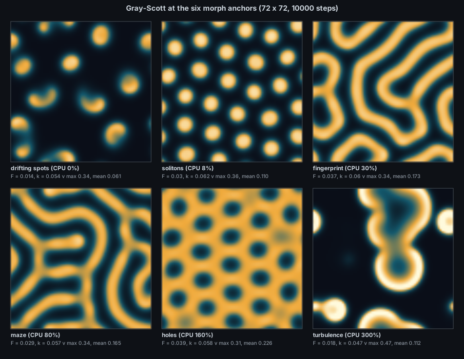
The six anchor points of the morph brief, simulated by docs/figures/reaction-diffusion-patterns.py (72 x 72 periodic dish, 10000 steps, activator $v$ shown). Left to right, top to bottom: drifting spots, solitons, fingerprint, maze, holes, turbulence.

History

Turing. Alan Turing published "The chemical basis of morphogenesis" in Philosophical Transactions of the Royal Society of London B in 1952, while at Manchester, and died in 1954. He asked how a ball of identical cells breaks symmetry, answered with the linear argument of section 1, and supplemented it with calculations on the Manchester computer. The paper was largely ignored by biologists for two decades. Hans Meinhardt and Alfred Gierer gave it a biologist's form in 1972 (a short-range activator and a long-range inhibitor), and the first laboratory Turing patterns in a chemical system waited until 1990, in a chlorite-iodide-malonic acid reaction (Castets and co-workers; Lengyel and Epstein, 1991).

Chemical clocks. The chemistry that made a reaction-diffusion dish plausible had its own trouble getting a hearing. Boris Belousov found an oscillating reaction in the early 1950s; reviewers rejected his manuscripts on the ground that a closed reaction could not oscillate, and he published only a brief abstract in a collection on radiation medicine. Anatol Zhabotinsky took the reaction up in the 1960s, and the Belousov-Zhabotinsky reaction became the standard example of chemical waves and spirals.

Gray and Scott. Peter Gray and Stephen Scott studied the autocatalytic step $A + 2B \to 3B$ in a stirred reactor at Leeds (Chemical Engineering Science, 1983 and 1984). In 1993 John Pearson of Los Alamos put the same two equations on a lattice, with a diffusivity ratio of two, and published "Complex patterns in a simple system" in Science: spots that divide, stripes, mazes, pulsing and chaotic regions in a single parameter plane of feed and kill. He labelled the regions with Greek letters. A notable point of his paper, which section 3 reproduces, is that for this diffusivity ratio the patterns are not classical Turing patterns. Karl Sims' web tutorial (2013) and Robert Munafo's xmorphia pages carried the map to a wide audience.

1. Theory: Turing's argument

Alan Turing, "The chemical basis of morphogenesis" (Philosophical Transactions of the Royal Society of London B 237, 1952), asked how a ball of identical cells could break symmetry. His answer: let $n$ chemicals (morphogens) react locally and diffuse, and look at a uniform steady state. If the state is stable against uniform perturbations but unstable against some spatially periodic ones, a pattern with a preferred wavelength grows out of noise. Diffusion, normally the great smoother, is the destabiliser.

1.1 The two-species system

$$ \partial_t u = D_u \nabla^2 u + f(u,v), \qquad \partial_t v = D_v \nabla^2 v + g(u,v). $$

Let $(u^, v^)$ satisfy $f = g = 0$ and let

$$ J = \begin{pmatrix} f_u & f_v \ g_u & g_v \end{pmatrix}_{(u^_,v^_)}, \qquad D = \begin{pmatrix} D_u & 0 \ 0 & D_v \end{pmatrix}. $$

Perturb the state by $\delta w = \varepsilon, e^{\lambda t}, e^{i \mathbf{q}\cdot\mathbf{x}}$. The Laplacian turns into $-q^2$, and the linearised equation becomes an eigenvalue problem,

$$ \lambda, \delta w = (J - q^2 D), \delta w . $$

The growth rate $\lambda(q)$ is the larger root of $\lambda^2 - \operatorname{tr}(J - q^2 D),\lambda + \det(J - q^2 D) = 0$.

1.2 The three conditions

1. Stable without diffusion ($q = 0$): $\operatorname{tr} J < 0$ and $\det J > 0$.
2. Trace stays negative with diffusion. $\operatorname{tr}(J - q^2 D) = \operatorname{tr} J - q^2 (D_u + D_v)$ is always more negative than $\operatorname{tr} J$, so a complex pair can never cross into instability through the trace. Stability can only be lost by a real eigenvalue crossing zero, that is by $\det(J - q^2 D) < 0$.
3. Expand the determinant. With $J - q^2 D = \begin{pmatrix} f_u - D_u q^2 & f_v \ g_u & g_v - D_v q^2 \end{pmatrix}$,

$$ h(q^2) \equiv \det(J - q^2 D) = D_u D_v, q^4 - \left(D_u g_v + D_v f_u\right) q^2 + \det J . $$

$h$ is a parabola in $q^2$ that opens upward and starts positive ($h(0) = \det J > 0$). It dips below zero for some $q$ exactly when

$$ D_u g_v + D_v f_u > 0 \qquad\text{and}\qquad \left(D_u g_v + D_v f_u\right)^2 > 4, D_u D_v \det J . $$

At threshold the critical wavenumber is $q_c^2 = \dfrac{D_u g_v + D_v f_u}{2 D_u D_v} = \sqrt{\dfrac{\det J}{D_u D_v}}$, and the pattern's wavelength is $2\pi/q_c$. Because $f_u + g_v < 0$ (condition 1) but $D_u g_v + D_v f_u > 0$, $f_u$ and $g_v$ must have opposite signs: one species feeds itself, the other damps itself, and the damped one must diffuse faster. That is Turing's "local activation, long-range inhibition" in two lines of algebra. With equal diffusivities the second inequality can never hold.

1.3 The biology it was built for

Gierer and Meinhardt (1972) turned the argument into a concrete activator-inhibitor model of biological patterning (Kybernetik 12). Kondo and Asai (1995, Nature 376) saw stripes on the marine angelfish Pomacanthus migrate and rearrange in the way a reaction-diffusion simulation predicts; Kondo and Miura (2010, Science 329) review the evidence. The first laboratory Turing patterns in a chemical system appeared in the 1990s (Castets et al. 1990, Physical Review Letters 64; Lengyel and Epstein 1991, Science 251). Whether any given animal pattern is "really" Turing's mechanism is an open empirical question; the mathematics does not depend on the answer.

2. Theory: the Gray-Scott model

The Gray-Scott model (Gray and Scott 1983, 1984, in Chemical Engineering Science, for the autocatalytic reaction $A + 2B \to 3B$, $B \to C$ in a stirred reactor) is, with $u$ the substrate $A$ and $v$ the autocatalyst $B$:

$$ \partial_t u = D_u \nabla^2 u - u v^2 + F,(1 - u), \qquad \partial_t v = D_v \nabla^2 v + u v^2 - (F + k), v . $$

$F$ is the feed rate (substrate refilled toward $u = 1$, and everything washed out at rate $F$) and $k$ is the kill rate (the extra removal of $B$). Pearson, "Complex patterns in a simple system" (Science 261, 1993), integrated it on a square lattice, found that the $(F, k)$ plane is cut into regions of qualitatively different long-term patterns, and labelled them with Greek letters; Karl Sims' reaction-diffusion tutorial and Robert Munafo's xmorphia popularised the map.

2.1 Fixed points

The trivial state $(u, v) = (1, 0)$ always exists. Its Jacobian is diagonal, $\operatorname{diag}(-F, -(F+k))$, so it is linearly stable for every $F, k > 0$. This is the key to everything below: the dish never develops a pattern from the trivial state by Turing's mechanism. A pattern needs a finite-amplitude seed.

Non-trivial states satisfy $u v = F + k$ and $F(1 - u) = u v^2$, which combine into $F u^2 - F u + (F + k)^2 = 0$:

$$ u^{\pm} = \tfrac12\left(1 \pm \sqrt{1 - 4 (F+k)^2 / F}\right), \qquad v = \frac{F + k}{u}. $$

They exist only if $F \ge 4(F+k)^2$, i.e. below the saddle-node curve

$$ k_{sn}(F) = \tfrac12 \sqrt{F} - F , $$

which peaks at $F = k = 1/16 = 0.0625$.

2.2 Linearisation at a non-trivial state

Using $u v = F + k$ the Jacobian simplifies to

$$ J = \begin{pmatrix} -v^2 - F & -2(F+k) \ v^2 & F + k \end{pmatrix}, \qquad \operatorname{tr} J = k - v^2, \qquad \det J = (F + k)(v^2 - F). $$

So the state loses stability to oscillations (a Hopf bifurcation) where $v^2 = k$. Substituting $v^2 = k$, $u = (F+k)/\sqrt{k}$ into the fixed-point equation gives $F^2 + F(2k - \sqrt{k}) + k^2 = 0$, hence the Hopf curve (the root with $F < k$, where $\det J > 0$)

$$ F_H(k) = \tfrac12\left[\sqrt{k} - 2k - \sqrt{k,(1 - 4\sqrt{k})}\right], \qquad k < 1/16 . $$

It meets the saddle-node curve at $F = k = 1/16$.

2.3 Diffusivities and the lattice

In lattice units (grid spacing 1, time step $\Delta t = 1$) the diffusivities that the isotop brief gives for the 5-point stencil are $D_u = 0.2097$, $D_v = 0.105$, ratio 2. They equal Pearson's continuum values $2\times10^{-5}$ and $10^{-5}$ divided by $(2.5/256)^2$ ($2\times10^{-5} / 9.54\times10^{-5} = 0.2097$); I believe that is Pearson's domain and grid, but have not checked the paper (unverified). The 9-point kernel the brief also mentions (0.2 on edges, 0.05 on corners, $-1$ at the centre) has Fourier symbol $\hat L_9(q_x, q_y) = 0.2(2\cos q_x + 2\cos q_y) + 0.05\cdot 4 \cos q_x\cos q_y - 1$, which along an axis is $-0.6,(1 - \cos q) = 0.3 \times(-2(1 - \cos q))$. The 5-point symbol along an axis is $-2(1-\cos q)$. So the 9-point kernel diffuses $0.3\times$ as fast per unit coefficient, and $D = 0.699, 0.35$ with it equals $D = 0.2097, 0.105$ with the 5-point stencil, as the brief says. The 9-point kernel is more isotropic: expanding the symbols, the 5-point stencil is $-q^2 + (q_x^4 + q_y^4)/12 + O(q^6)$ with an anisotropic fourth-order term, whereas the 0.2/0.05 kernel is $-0.3,q^2 + (q_x^2 + q_y^2)^2/40 + O(q^6)$, whose fourth-order term is rotation invariant. Its anisotropy only appears at sixth order, which is why Sims uses it.

Explicit Euler is stable for the diffusion part when $D,\Delta t,\max|\hat L| \le 2$: the 5-point symbol reaches $-8$ so $D \le 0.25$ (we have $0.2097$); the 9-point symbol reaches $-1.6$ so $D \le 1.25$ (we have $0.699$). Reaction terms are non-stiff at these rates.

3. Where the patterns live: the $(F, k)$ plane

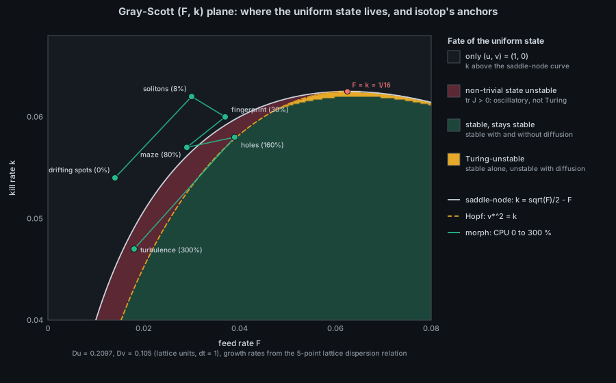
docs/figures/reaction-diffusion-plane.py. Each pixel is classified from the lower-$u$ non-trivial state, with the 5-point lattice dispersion relation at $D_u = 0.2097$, $D_v = 0.105$. Aqua line: the path of the morph view's CPU interpolation, anchors dotted.

What the figure shows, and what it does not:

Region	Shown colour	Meaning
$k > k_{sn}(F)$	dark	only the trivial state exists (and it is stable)
between saddle-node and Hopf	red-brown	a non-trivial state exists but is unstable without diffusion ($\operatorname{tr} J > 0$)
right of the Hopf curve	green	the non-trivial state is stable, with and without diffusion
a thin sliver near $F \approx 0.05$ to $0.08$, hugging $k \approx 0.062$	amber	Turing-unstable: stable alone, unstable with diffusion (about 0.6 % of the plotted area)

The six isotop anchors, checked against these curves:

Anchor	CPU %	$F$	$k$	$k_{sn}(F)$	Non-trivial state?
drifting spots	0	0.014	0.054	0.0452	none ($k > k_{sn}$)
solitons	8	0.030	0.062	0.0566	none
fingerprint	30	0.037	0.060	0.0592	none
maze	80	0.029	0.057	0.0561	none
holes	160	0.039	0.058	0.0597	exists, lower branch $\operatorname{tr} J = +0.0011$: just left of the Hopf curve ($F_H(0.058) = 0.0394$)
turbulence	300	0.018	0.047	0.0491	exists, lower branch $\operatorname{tr} J = +0.0172$: unstable focus ($F_H(0.047) = 0.0219$)

The conclusion is worth stating bluntly. None of the six isotop anchors is a classical Turing pattern. Four have no non-trivial uniform state at all; the trivial state is the only uniform state and is stable, so the spots, solitons, fingerprints and mazes grow from finite-amplitude nuclei by front propagation (a spot grows, splits, and the fronts fill the dish). The other two have an unstable non-trivial state. The name "Turing patterns" is therefore a loose label for "reaction-diffusion patterns of an activator-substrate system"; the genuinely linear Turing region exists (amber, at $F \gtrsim 0.05$) but isotop's CPU path does not go there. This also explains two rules in the specified view: a new patch is seeded with nuclei, and a live patch whose $\max v$ falls below $0.05$ is reseeded, because once $v \equiv 0$ the stable trivial state can never regrow a pattern on its own.

3.1 The dispersion relation, worked at one point

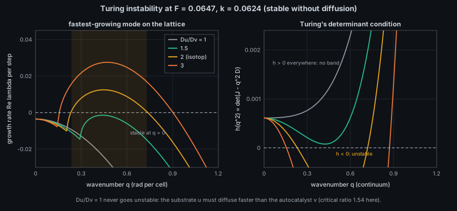
docs/figures/reaction-diffusion-dispersion.py, inside the amber sliver at $(F, k) = (0.0647, 0.0624)$.

At this point $u^* = 0.4822$, $v^* = 0.2636$, $\operatorname{tr} J = -0.00709$, $\det J = 6.09\times10^{-4}$. The critical diffusivity ratio is $D_u/D_v = 1.54$. With the ratio set to 1 the fastest mode decays; at 1.5 it still decays (barely); at the isotop ratio 2 the band $q \in [0.236, 0.730]$ rad per cell grows, fastest at $q = 0.448$ (a wavelength of about 14 cells) with rate $0.0125$ per step, so the e-folding time of the pattern amplitude is about 80 steps. The kink in each curve is where the eigenvalue pair turns from complex to real.

4. Behaviour you can rely on

• Wavelength is set by the chemistry, not the dish. Enlarging the dish adds more spots or stripes, not larger ones.
• Time scale is thousands of steps. In the patterns figure, 10000 steps at $\Delta t = 1$ are needed before the six anchors look settled on a 72 x 72 dish; maze and turbulence continue to evolve.
• Starvation is fast. Switching a settled periodic 64 x 64 test patch to $F = 0$, $k = 0.06$ (the exit rule of the specified view) drops $\max v$ from $0.3$ to $0.4$ to below $0.01$ in under 100 steps for every anchor state I tried (spots, solitons, maze, holes, turbulence): with $F = 0$ the substrate is never replenished, the term $v(uv - k)$ turns negative, and $v$ decays at about $k$ per step. In a real dish the edge of the patch is coupled to live neighbours, so the observed starvation near borders can be slower. This test is a patch alone; it is not a measurement of any isotop code.
• Noise-free runs are deterministic. The figure scripts seed with a splitmix64 stream, the same family as isotop's simulation::Rng; two runs are bit-identical.

5. What this means for isotop

Everything in this section is the specified design of Planned-Morph (issue #50); no src/morph.rs exists yet.

• The dish is a fixed 256 x 256 grid with zero-flux edges (the prototype in docs/mockups/code/morph.py wraps instead; the issue wins), Sims's 9-point kernel with $D_u = 0.699$, $D_v = 0.35$, $\Delta t = 1$, stepped by simulation::FixedStep at 240 steps per second of view time.
• Per-cell $F$ and $k$ come from each process's CPU through the anchor table above, interpolated on $\log(1 + \text{cpu})$ and blurred with a Gaussian of $\sigma \approx 1.5$ cells across patch borders.
• The picture lets a viewer infer only a coarse ordering: more CPU moves the patch along the aqua path in the plane, from isolated spots through stripes to holes and boiling. It does not let a viewer read CPU off the pattern, because the mapping from $(F, k)$ to morphology is not monotone in any single feature (the path doubles back in $F$ between 160 % and 300 %).

6. Try it

python3 docs/figures/reaction-diffusion-plane.py        # about 1 s
python3 docs/figures/reaction-diffusion-dispersion.py   # about 1 s, prints the numbers quoted above
python3 docs/figures/reaction-diffusion-patterns.py     # about 3 minutes (single process pool of 4)

The simulator is docs/figures/rdsim_w8.py (explicit Euler, 5-point stencil, periodic, standard library only).

7. Where in the code

• Nothing in src/ implements reaction-diffusion yet. The planned module is src/morph.rs (Planned-Morph).
• The nearest existing precedent for a pure grid simulation is src/medium.rs (the Ripple wave equation, see Math-Wave-Equation); the fixed-step clock is simulation::FixedStep in src/simulation.rs (see Theory-Simulation-Toolkit).
• The prototype with the anchor table and the power-diagram patches is docs/mockups/code/morph.py (numpy and scipy; reference only).

8. Variations and open questions

• Run the six anchors with the 9-point kernel and compare the wavelength and the isotropy of the spot lattice.
• Find the isotop CPU path's nearest approach to the Turing sliver and ask whether a different anchor table would pass through it.
• Measure how many dt-1 steps a 256 x 256 dish needs to settle a maze from 8 nuclei, and compare with the 1500 settle steps specified.
• Zero-flux versus periodic edges: does clamping change which pattern a small patch picks?

References

• A. M. Turing, "The chemical basis of morphogenesis", Philosophical Transactions of the Royal Society of London B 237 (1952) 37-72.
• A. Gierer and H. Meinhardt, "A theory of biological pattern formation", Kybernetik 12 (1972) 30-39.
• P. Gray and S. K. Scott, "Autocatalytic reactions in the isothermal, continuous stirred tank reactor: isolas and other forms of multistability", Chemical Engineering Science 38 (1983); and "... oscillations and instabilities in the system A + 2B -> 3B; B -> C", Chemical Engineering Science 39 (1984).
• J. E. Pearson, "Complex patterns in a simple system", Science 261 (1993) 189-192.
• S. Kondo and R. Asai, "A reaction-diffusion wave on the skin of the marine angelfish Pomacanthus", Nature 376 (1995) 765-768; S. Kondo and T. Miura, "Reaction-diffusion model as a framework for understanding biological pattern formation", Science 329 (2010) 1616-1620.
• K. Sims, "Reaction-Diffusion Tutorial" (web page, 2013); R. Munafo, "xmorphia" (web pages).
• J. D. Murray, Mathematical Biology II: Spatial Models and Biomedical Applications (Springer, 3rd ed. 2003), the chapter on pattern formation.