Planned Die

Planned: Die

Planned, not yet implemented. Specified in docs/briefs/views-2026-10.md and tracked in issue #56.

The CPU die seen from above in FLIR ironbow false colour: a schematic floorplan of P-cores, E-core clusters, cache slices, an integrated GPU and the uncore, a heat field that blooms over working cores and diffuses across the silicon, processes as small hot points over the core each last ran on, a core outline that flashes when it throttles, and a readout of temperatures and package power where the machine lets isotop read them. This page is the design, with the physics of infrared thermography, what the kernel exposes about CPU temperature and power, the heat equation the view integrates and its numerics, and a clear statement of which parts are measurement and which are a model.

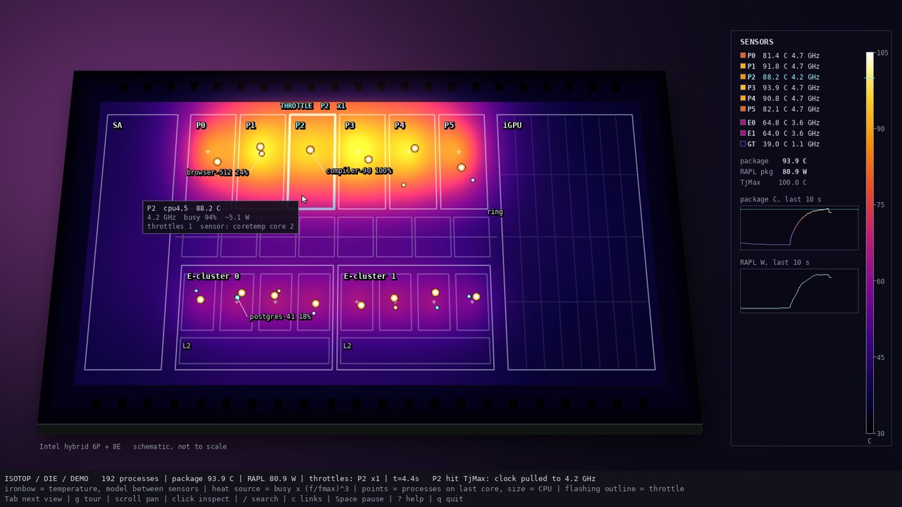
docs/mockups/die.jpg, from the prototype docs/mockups/code/die.py (a 6P + 8E hybrid floorplan under a synthetic compile load, one P-core reaching TjMax). A visual target, not an isotop render.

1. The system being modelled

1.1 Seeing heat

Every object above absolute zero radiates. Planck's law gives the power per unit area and wavelength of an ideal blackbody at temperature $T$,

$$ M_\lambda(T) = \frac{2\pi h c^2}{\lambda^5},\frac{1}{e^{hc/\lambda k_B T} - 1}, $$

whose peak moves with temperature by Wien's displacement law, $\lambda_{max} T = b = 2897.77\ \mu\text{m·K}$. At 300 to 390 K the peak is at 9.7 to 7.4 $\mu$m, in the long-wave infrared (LWIR, about 8 to 14 $\mu$m), where thermal cameras like FLIR's work and the atmosphere is transparent. Integrating Planck's law (the figure's script) the 8 to 14 $\mu$m band carries 38 to 39 % of the total exitance across that range, and its exitance rises as $T^{4.2}$ near 330 K, so a 1 % rise in absolute temperature (3.3 K) raises the band radiance by about 4.2 %: that is the sensitivity a thermographer exploits.

A real surface is not a blackbody. Its emissivity $\varepsilon \le 1$ scales what it emits, and for an opaque surface the camera sees $\varepsilon M(T) + (1 - \varepsilon)M(T_{refl})$, so a shiny low-emissivity surface looks cooler than it is and reflects its surroundings. Silicon is a hard case (its emissivity depends on doping, temperature and surface finish, and lightly doped silicon is partly transparent in the infrared), which is why thermal images of bare dies are usually taken with a coating or a calibrated emissivity. FLIR images of a delidded CPU under load are the visual reference for this view; they are what the false colours imitate, not what the view measures.

1.2 Why ironbow

The ironbow palette runs black, deep blue, purple, magenta, red, orange, yellow and white as temperature rises. It is a good palette for a quantity with a natural zero and a scary top: its luma rises monotonically (computed from the prototype's stops with Rec. 709 weights, from 0 at the cold end to 255 at white, in the figure), so ordering survives greyscale, and hot is the brightest, an instant read. Rainbow ("jet") palettes lack that property and mislead (Borland and Taylor 2007, "Rainbow color map (still) considered harmful"). The view maps 30 degrees C to TjMax + 5 degrees (TjMax is 100 degrees when unknown) onto an in-tree gradient table, so 30 to 105 degrees C by default.

1.3 What the machine exposes

• Per-core and package temperature. On Intel the digital thermal sensor of each core reports the margin below TjMax (the maximum junction temperature, commonly 100 degrees C, SKU dependent); the coretemp hwmon driver computes Core N = TjMax - margin, with 1 degree resolution, plus a Package id P sensor. On AMD the k10temp driver gives Tctl (a control temperature that can carry a fixed offset on some parts), Tdie, and on parts with chiplets Tccd per core complex die. Package-only fallbacks exist for ARM and some virtual machines (the hwmon chips cpu_thermal and soc_thermal, and the x86_pkg_temp thermal zone).
• Throttle counts. On Intel, /sys/devices/system/cpu/cpuN/thermal_throttle/core_throttle_count and package_throttle_count increase when the hardware throttled the core or the package for thermal reasons (PROCHOT). Intel only.
• Package power: RAPL. Intel's (and, for the AMD parts that offer it, AMD's) Running Average Power Limit exposes an energy counter through the powercap sysfs tree, /sys/class/powercap/intel-rapl:N/energy_uj, in microjoules; power is the delta over time. With the typical energy unit of 61 microjoules the 32-bit counter wraps at about 262 kJ, after about 44 minutes at 100 W, so the wrap must be handled. Since 2020, after the PLATYPUS power side-channel attacks (Lipp et al., IEEE S&P 2021), most kernels make the energy counter readable by root only: isotop never escalates privilege, so on such kernels it reports Measured::Unreadable and the view says so.
• Topology. /sys/devices/system/cpu/cpu*/topology/* (package, die, core id, cluster id, core_cpus_list, which lists SMT siblings) and cache/index2|3/shared_cpu_list (how LP E-cores on tiled parts show as their own cluster).
• Frequency and DVFS. Dynamic CMOS power is $P = \alpha C V^2 f$; with dynamic voltage and frequency scaling $V$ tracks $f$ roughly linearly, so $P \propto f^3$ across the DVFS range, which is the proxy the view uses; leakage grows exponentially with temperature and adds a feedback that thermal throttling and frequency pull-down exist to stop.

1.4 What macOS cannot read

macOS exposes no unprivileged per-core temperatures, throttle counts or package power: the sensors are behind the SMC or the private HID event system, and powermetrics needs root. B12 therefore reports temperature, throttle counts and package power in Snapshot.missing on macOS, and the view is available in a degraded form: a generic Apple floorplan built from P/E core kinds and the measured cluster clocks, the field in relative heat, process points on their P or E cluster by performance_share (macOS reports no last CPU). Note that the brief said Linux only with a one-line explanation elsewhere; the issue overrides it and the view conventions list it as available on macOS.

History

Heat was first seen as light by accident. In 1800 William Herschel passed sunlight through a prism and laid thermometers with blackened bulbs along the spectrum to see how much heat each colour carried. The temperature rose toward the red end and was highest in the dark just beyond it, from which he concluded that sunlight contains invisible rays; he published the experiments in the Philosophical Transactions of the Royal Society. The name infrared came later. Wien's displacement law (1896) and Planck's law, which says how much a body at a given temperature radiates at each wavelength (1901), followed a century on; both are in the references.

The thing being imaged is younger. Jack Kilby at Texas Instruments conceived the integrated circuit in July 1958 and had a working oscillator on a single piece of germanium by September; his patent was filed in February 1959. Robert Noyce at Fairchild filed in July 1959 for a version in which the interconnects were laid down as a film over an oxide layer, which is what made manufacture practical. Accounts differ on how to share the credit; the two companies settled by cross-licensing in 1966. A die is one such circuit cut from its wafer; this page treats it as a rectangle of silicon with a heat source in it.

Dealing with the heat in hardware is younger still. The Pentium 4 carried a thermal monitor that slowed the clock when the core reached a trigger temperature. Tom's Hardware published a widely discussed test in which the heatsink was removed from a running Pentium 4 and from running Athlons (I did not confirm the article's date; forum posts place it around 2001). The Athlons failed within fractions of a second; the Pentium 4 slowed down, and Quake III Arena kept running, more slowly. Supporters of AMD disputed the test, and a counter-video showed a later Athlon surviving.

2. Theory: the heat equation on a die

Fourier's law $\mathbf{q} = -k\nabla T$ and conservation of energy, $\rho c_p,\partial_t T = \nabla!\cdot(k\nabla T) + q_v$, give for uniform $k$

$$ \partial_t T = \kappa\nabla^2 T + \frac{q_v}{\rho c_p}, \qquad \kappa = \frac{k}{\rho c_p}. $$

For silicon (textbook values $k \approx 148$ W/m·K, $\rho = 2329$ kg/m$^3$, $c_p \approx 705$ J/kg·K) $\kappa \approx 9.0\times10^{-5}$ m$^2$/s $= 90$ mm$^2$/s: heat crosses a 2 mm core in $L^2/\kappa \approx 44$ ms. The view adds a sink, the heat that leaves into the package, heat spreader and cooler, as a relaxation toward ambient with time constant $\tau$:

$$ \frac{\partial T}{\partial t} = \kappa\nabla^2 T + \text{gain}\cdot P(x,y) - \frac{T - T_{amb}}{\tau}. $$

2.1 Specified constants, and what they mean

The issue fixes a 192 x 96 grid, $\kappa = 90$ cells$^2$/s and $\tau = 2.0$ s, with an explicit 5-point step $T \leftarrow T + h,[\kappa\nabla^2T + \text{gain},P - (T - T_{amb})/\tau]$ and $h = 0.2/\kappa$. Three things follow.

• The numbers are the model's, not silicon's. If the grid spans a 20 mm x 10 mm die, a cell is 0.104 mm and silicon's $\kappa$ would be about 8300 cells$^2$/s, 92 times the view's 90. The view's lateral spreading is therefore about 90 times slower than silicon's, tuned for visibility; real silicon equilibrates laterally in milliseconds, far faster than a frame. The time constant $\tau = 2$ s is a package-scale thermal inertia (heat spreader, cooler), not the silicon's. Real CPU thermal response is a ladder of resistor-capacitor stages (die in milliseconds, spreader around a second, cooler over tens of seconds) which the single $\tau$ stands in for.
• Stability. For the explicit 5-point scheme the von Neumann amplification factor of a Fourier mode is $g = 1 - 4r\left(\sin^2\tfrac{q_x}{2} + \sin^2\tfrac{q_y}{2}\right) - h/\tau$ with $r = \kappa h$ (unit cell spacing), whose worst mode (the checkerboard, $\sin^2 = 1$ in both directions) gives $g = 1 - 8r - h/\tau$; $|g| \le 1$ requires $r \le 1/4$, the CFL limit for two dimensions. With $h = 0.2/\kappa$, $r = 0.2$: stable, at 80 % of the limit, and the sink adds a stabilising $-h/\tau$. A frame step above the limit would blow up as $(1 - 8r)^n$: the issue clamps the frame $dt$ to $[0, 0.25]$ s and takes fixed steps of $h = 2.2$ ms through simulation::FixedStep, 112 steps at most per frame. A cold start pre-rolls $3\tau = 6$ s, 2700 steps over 18,432 cells, 50 million cell updates once; at 60 fps a frame needs 7.5 steps, about 138 thousand cell updates.
• Conservation. With zero-flux (clamped) edges the discrete Laplacian sums to zero, so without sources and sinks $\sum T$ is conserved exactly (the issue's test heat_is_conserved_without_sinks_or_sources).

2.2 The screened response

With a sink the steady response to a point source is not the long-tailed $\ln r$ of the pure heat equation in two dimensions but a screened one: $\kappa\nabla^2 T - T/\tau = -q,\delta$ has the solution

$$ T(r) = T_{amb} + \frac{q}{2\pi\kappa},K_0!\left(\frac{r}{\lambda}\right),\qquad \lambda = \sqrt{\kappa\tau}, $$

with $K_0$ the modified Bessel function of the second kind, which falls off as $e^{-r/\lambda}/\sqrt{r}$ beyond $\lambda$. The screening length $\lambda = \sqrt{\kappa\tau} = \sqrt{90\times2} = 13.4$ cells sets how far a hot core's glow reaches: the "bloom" is a $K_0$ halo of that radius. The figure checks it: a point source on a 64 x 64 grid with $\kappa = 22.5$, $\tau = 2$ ($\lambda = 6.7$ cells) settles to a profile that matches $K_0(r/\lambda)$ to within 1 % between 3 and 19 cells (ratio 0.99 to 1.00).

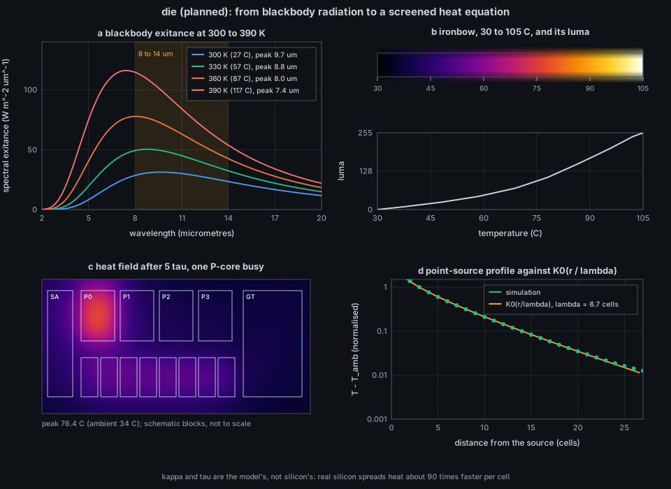
docs/figures/die-thermal.py (about 4 s of pure Python). (a) Blackbody exitance at 300 to 390 K with the 8 to 14 micrometre band; (b) the prototype's ironbow stops and their luma; (c) the specified heat equation on a toy hybrid floorplan at half resolution, one P-core busy, gain calibrated so that one P-core at full proxy settles 40 K above ambient, as in the prototype (peak 76.4 degrees C including its neighbours); (d) the point-source profile against $K_0$.

2.3 Nudging: sensors as ground truth

Between sensors the field is a model. The issue makes each sensor a ground truth that pulls the model toward it: a Gaussian footprint of radius 4 cells around the sensor's location (Intel per-core sensors at P-core hotspots, AMD per-CCD sensors at CCD centres), toward the reading, with weight $1 - e^{-\Delta t/0.25}$ per step; the package sensor shifts the whole field so that the hottest core block matches it; and $T_{amb}$ is the lowest sensor reading over the last 60 s minus 5 K. This is nudging (Newtonian relaxation), the simplest of the data-assimilation methods that numerical weather prediction uses to keep a model near its observations; a Kalman filter would weight model and measurement by their uncertainties and the nudging weight is a fixed time constant instead. B12 samples thermal sensors on the existing 2-second background pass, so readings change at most every 2 s and the field is pulled to each new value within about 0.25 s: the picture steps.

3. Mapping

Visual element	Measured quantity (source)	Transform
Heat field colour	the model, nudged by sensors (B12 Snapshot.thermal.sensors)	$T$ from 30 degrees C to TjMax + 5 through the ironbow table, one P3 field draw; relative units and a relative colour bar when no sensor exists
Heat source per core block	Cpu.busy and Cpu.mhz of the block's logical CPUs	$P = \text{busy},(f/f_{max})^3$ with $f_{max}$ = cpuinfo_max_freq where B12 gives it, else the running maximum of the measured clock; normalised to RAPL watts with a 2 s EMA when RAPL is readable
Block layout	topology from core_cpus_list (B12)	four generators: Intel hybrid, Intel tiled (LP E-cores their own cluster), AMD CCDs plus IOD, generic core grid; SMT siblings share a block; schematic, not to scale (a caption says so on screen)
Process point	Process.core (last CPU; Linux only) and Process.cpu	small sphere sized by CPU over the block of that CPU, offset from Rng::for_identity, so it stays put while the process stays on the core
Core outline flash	core_throttle_count increments	1.4 s per increment; status throttles: P2 x1
Readout panel	sensors, TjMax, RAPL watts	colour bar, per-block readouts, two 60 s sparklines (package degrees C, RAPL W) fed by the per-sample record hook
Substrate, pins, L3, L2, iGPU, system agent	none	schematic context, unmeasured
Sky, die slab	none	decorative

4. Design: how isotop will realise it

• Module. src/die.rs with state Die, which implements views::ViewModule, and one ViewInfo::new(name, title, backdrop, build) row at the end of views::REGISTRY: Backdrop::Dusk, B12's sources declared through S6, no view-local keys; hover and click on core blocks through B9's non-process pickables. The owner grid names the core block under each cell, NONE elsewhere.
• Heat core. Explicit 5-point step, 192 x 96, $\kappa = 90$ cells$^2$/s, $\tau = 2.0$ s, FixedStep with $h = 0.2/\kappa$; gain calibrated as in the prototype; at 1080p the simulation stays under 2 ms per frame and the field is one P3 draw, never a triangle pair per cell. At --processes 1000 the points are 1000 small spheres.
• Power proxy. As in the mapping table. The proxy is a stated proxy, and the README says the field between sensors is a model.
• Demo. The demo keeps its 16 CPUs and presents them as an Intel hybrid with 4 SMT P-cores (cpu0 to cpu7) and 8 E-cores in two clusters of four (cpu8 to cpu15); topology, per-core sensors (a first-order lag of the proxy), the package sensor, TjMax, RAPL and one P-core that crosses TjMax and throttles once per 40 s cycle are synthesized deterministically in --time, extending B12's demo.
• Dependencies (ROADMAP index): P1, P2, S1, P3, B9, B12, S2, S6. In the current tree: P1, P2, S1, S2, S6, B9 and P3 (src/render/field.rs) are merged; B12 (thermal and topology) is not.
• Platforms. Linux with hwmon: the full view in degrees C. Linux without hwmon (VMs, CI): relative units, colour bar labelled relative, and the strip names the missing temperature source followed by field is model only. RAPL unreadable: RAPL n/a (root only) and the proxy stays unscaled. macOS: available, degraded (section 1.4). The view is never a "not supported" screen.
• No plugin system. Compile-time module and REGISTRY row.

5. Reading the picture

• Measured: the temperature at each sensor (at 1 degree resolution, at most every 2 s), throttle events, package power if readable, the clock and busy fraction of each CPU, and which CPU a process last ran on.
• Derived: everything between the sensors. The field is a model with specified constants that are 90 times too slow for silicon; a spot of colour at a place where no sensor sits is the model's idea, not the chip's. The power proxy $\text{busy},(f/f_{max})^3$ is a proxy.
• Process points show where a process last ran, not where heat was made: Linux reports the last CPU in stat, a snapshot at the sample.
• Decorative: the die slab, sky and sensor panel chrome.
• Cannot infer: a junction hot spot (an execution unit's temperature is not visible to a core sensor), hot spots of the iGPU or uncore (no sensor), absolute accuracy on AMD where Tctl can carry an offset, or throttling that the counters do not count (power-limit throttling is not thermal throttling).
• Resolution limits: 1 degree sensor resolution, a 2 s sample cadence, a 192 x 96 grid with cells of order 0.1 mm if the die were to scale (it is not).
• A flash is a counter increment, not a measurement of duration: 1.4 s of outline per increment however long the throttle lasted.

6. Try it

Nothing runs in isotop yet. When the view lands:

./target/release/isotop --demo --view die --time 12 --width 1600 --output /tmp/die.png --renderer cpu

(Tab and the v picker reach it.) To see what a Linux machine offers today:

grep . /sys/class/hwmon/hwmon*/name
cat /sys/class/hwmon/hwmon*/temp*_label /sys/class/hwmon/hwmon*/temp*_input 2>/dev/null | head
cat /sys/devices/system/cpu/cpu0/thermal_throttle/core_throttle_count 2>/dev/null
cat /sys/class/powercap/intel-rapl:0/energy_uj      # may need root
python3 docs/figures/die-thermal.py                  # this page's figure

7. Where in the code

Existing: model::Cpu (busy, mhz, kind), CoreKind, Process.core in src/model.rs; palette::core_color in src/palette.rs; simulation::FixedStep and Rng::for_identity in src/simulation.rs; terminal::clean_text; Thing, Card in src/render.rs; the field primitive (Field, Relief, Frame::field) in src/render/field.rs. Planned: src/die.rs, B12's src/platform/linux/thermal.rs (hwmon, topology, throttle counts, RAPL) and its macOS topology in src/platform/macos/logic.rs, parse_cpu_list, which B4 already put in src/platform/linux/counters.rs. The prototype is docs/mockups/code/die.py (numpy, scipy, OpenCV; reference only).

8. Variations and open questions

• Replace the single $\tau$ by a two-stage package model (spreader and cooler) and see whether throttle cycles look more like the real thing.
• Rescale $\kappa$ to silicon's value and the grid to real die dimensions, then show the field at a sub-frame time step for sub-second transients.
• Calibrate the gain per machine by a least-squares fit of the proxy to the per-core sensors over a run (a Kalman filter instead of nudging).
• Show the sensor's margin to TjMax (what Intel reports) instead of absolute degrees.
• Show RAPL power limits (PL1, PL2) and the time window when readable.
• Add the iGPU and memory controller as heat sources from their own counters where available.

9. References

• W. Herschel, "Experiments on the refrangibility of the invisible rays of the Sun", Philosophical Transactions of the Royal Society of London (1800).
• M. Planck, "Ueber das Gesetz der Energieverteilung im Normalspectrum", Annalen der Physik 4 (1901) 553-563; W. Wien, "Ueber die Energievertheilung im Emissionsspectrum eines schwarzen Koerpers", Annalen der Physik 58 (1896) 662-669.
• J. P. Holman, Heat Transfer (McGraw-Hill), and F. P. Incropera and D. P. DeWitt, Fundamentals of Heat and Mass Transfer (Wiley), for emissivity, silicon properties and the heat equation.
• D. Borland and R. M. Taylor II, "Rainbow color map (still) considered harmful", IEEE Computer Graphics and Applications 27(2) (2007) 14-17.
• M. Lipp et al., "PLATYPUS: Software-based power side-channel attacks on x86", IEEE Symposium on Security and Privacy (2021).
• Linux kernel documentation for hwmon (coretemp, k10temp), powercap (RAPL) and thermal_throttle.
• Issue #56 and B12 (#39); docs/briefs/views-2026-10.md section 17; docs/VIEW_CONVENTIONS.md. See also Theory-Colour, Theory-Background-Sampler-and-Demand, Theory-Text-Safety.