Planned Canyon

Planned: Canyon

Planned, not yet implemented. Specified in docs/briefs/views-2026-10.md and tracked in issue #55.

A sunlit desert in isometric relief that changes over minutes and hours, and is saved between runs so that it keeps a record of the machine's history over days. Mesas rise where big processes live, rivers carve gorges where busy processes rain, alluvial fans and deltas spread in the colours of the processes whose rain carried the sediment, lakes fill the pits, and banded strata show in the canyon walls. The terrain is the one stateful view in the plan: it is not a picture of the current sample but an accumulation of everything the machine has done on each plot, and the design has to be honest about what such an accumulation can and cannot tell you. This page is that design, the geology it leans on (stratigraphy, the stream power law, droplet erosion), and a simulation with the specified constants.

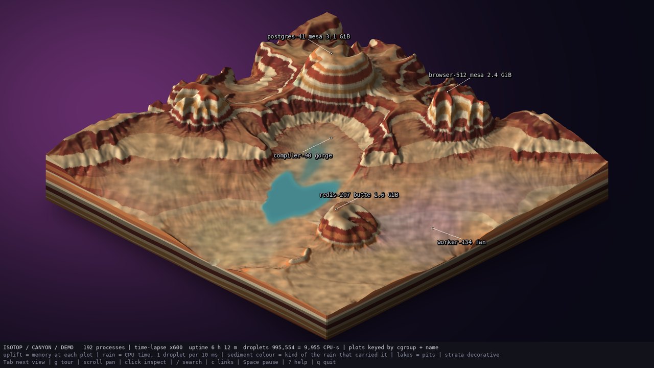
docs/mockups/canyon.jpg, from the prototype docs/mockups/code/canyon.py: a 256 x 256 heightfield after a synthetic demo day (6 h 12 m, 995,554 droplets). A visual target, not an isotop render.

1. The system being modelled

1.1 Stratigraphy and what a landscape remembers

Geology reads history from rock. Nicolas Steno (1669) formulated the first laws of stratigraphy: superposition (in an undisturbed sequence the oldest layer is at the bottom), original horizontality (sediments are laid down in horizontal layers) and lateral continuity (a layer extends until it thins or meets a barrier). James Hutton's unconformity at Siccar Point (1788) added that a sequence can be tilted, eroded and buried again, and Charles Lyell's cross-cutting relations that whatever cuts a layer is younger than it. A canyon is stratigraphy exposed by erosion: the walls show the layers, and the river that exposed them is the youngest feature.

The same reading does not carry over to isotop's canyon, and the difference is the most important thing on this page. The terrain stores a heightfield and a top layer of sediment: heights, a base level, per-cell sediment weight and colour, a total quantum count and per-plot carries. It does not store a stack of layers by time. The strata in the walls (colours and bands) are decorative, a function of height with a constant seed, drawn "so the walls read", and not a record of when anything happened. Steno's superposition does not hold in the model.

1.2 What the terrain does record

Think of the canyon as a low-pass filter with memory. Each CPU-second of a process falls as rain on its plot and moves material; each memory-GiB-hour of a process raises its plot; each hour of nothing relaxes everything toward base level. The surface is an integral of that history and, like real landscapes, it forgets: a short burst of rain cuts a small gully that later rain, deposition or relaxation may erase; a plot that has been idle for days relaxes back toward flat. This is the geological Sadler effect (Sadler 1981, Journal of Geology 89), the observation that apparent sediment accumulation rates fall as the time span of the measurement grows because the record is full of gaps at every scale. The terrain preserves long-lived, large signals (a service that runs for weeks and uses gigabytes) and loses short-lived, small ones.

History

Section 1.1 gives the older history of reading rock. The history of reading this rock begins in the nineteenth century. John Wesley Powell and nine volunteers left Green River Station, in Wyoming Territory, on 24 May 1869 and finished the passage through the Grand Canyon at the mouth of the Virgin River on 30 August 1869. After a small appropriation from Congress he made a second descent in 1871 and 1872, which ended at the mouth of Kanab Creek. His account, Explorations of the Colorado River of the West and Its Tributaries, appeared in 1875, and he revised and enlarged it in 1895 as Canyons of the Colorado.

The geology was worked out next. Clarence Dutton's Tertiary History of the Grand Cañon District (USGS Monograph 2, 1882, with an atlas, issued while Powell directed the Survey) is the source several accounts give for the name Great Unconformity, the surface where flat sedimentary layers sit on tilted older rock in the canyon walls; one source adds that Dutton named it without knowing the age of the rocks on either side, so the name does not measure the gap. Powell's own report contains a drawing of the contact.

The numerical history is shorter. Erosion by channels was modelled as a power law of drainage area and slope from the 1980s (Howard and Kerby 1983; Whipple and Tucker 1999), and by simulated droplets on a heightfield from the mid-2000s (Mei, Decaudin and Hu 2007; Beyer 2015); the view uses the second.

2. Theory

2.1 Stream power, and why landscapes are concave

The standard landscape-evolution model is the stream power law (Howard and Kerby 1983; Whipple and Tucker 1999, Journal of Geophysical Research 104): the height $h$ of a channel changes by uplift $U$, minus incision proportional to a power of the drainage area $A$ upstream and the local slope $S$, plus slow diffusion of hillslopes:

$$ \frac{\partial h}{\partial t} = U - K A^{m} S^{n} + D\nabla^2 h . $$

At steady state uplift and incision balance, $U = K A^m S^n$, giving

$$ S = \left(\frac{U}{K}\right)^{1/n} A^{-m/n}. $$

Slope falls as a power of drainage area with concavity $\theta = m/n$, typically 0.4 to 0.6: this is Flint's law (Flint 1974, Water Resources Research 10), which is why river profiles are concave-up, steep near the head and gentle near the mouth. Where $U$ is larger the channel is steeper (by $U^{1/n}$); a uniform uplift with no erosion makes a plateau; erosion without uplift makes a plain.

2.2 The droplet model

The specified view does not integrate the stream power law. It follows hydraulic erosion by droplets (Beyer 2015, a TU Munich bachelor thesis; a particle method in the tradition of Mei, Decaudin and Hu 2007 who simulated erosion with a shallow-water model on the GPU). Each droplet has a position, a direction, a speed, an amount of water and of carried sediment, and each step does the following on the bilinear heightfield:

1. Compute the bilinear height gradient $\nabla h$ at the position; update the direction $d \leftarrow d\cdot\text{inertia} - \nabla h,(1 - \text{inertia})$ and normalise (inertia 0.05: the droplet follows the slope almost exactly).
2. Step one cell along $d$ and take the height difference $\Delta h$.
3. The carrying capacity is $c = \max(-\Delta h,\ c_{min})\ v\ w\ \kappa$ with $\kappa = 4$ and $c_{min} = 0.0008$: a steeper, faster, wetter droplet carries more.
4. If the droplet carries more than its capacity, or is moving uphill, it deposits: $\min(\Delta h, s)$ going uphill, else $(s - c)\times0.3$, spread bilinearly to the four corners of the cell it left. Otherwise it erodes $\min((c - s)\times0.15,\ -\Delta h)$, taken from the cells under a brush of radius 3.
5. Update speed $v \leftarrow \sqrt{v^2 + \Delta h,g}$ with $g = 4$, water $w \leftarrow 0.99,w$ (evaporation 0.01); a droplet lives at most 70 steps.

These constants are those of the prototype and of the issue. Reading the algorithm as a scaling law (my own argument, not verified numerically): the number of droplets crossing a cell per unit time is proportional to the drainage area $A$ upstream, and each removes an amount proportional to $S,v,w$, so the incision rate scales like $A,S,v$, which corresponds to a stream power law with $m \approx 1$ and an $n$ between 1 and 1.5 (the speed $v$ grows with the square root of the drop). The droplet model reproduces the physics qualitatively (channels, gullies, fans, carved mesas) and not the numbers.

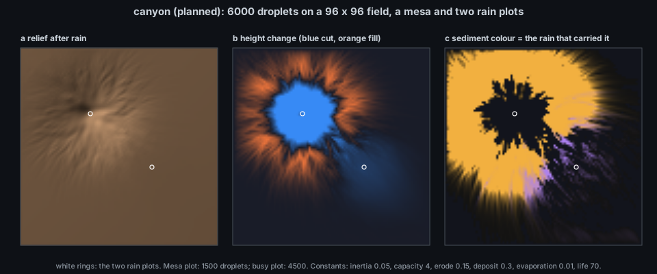
docs/figures/canyon-erosion.py (about 15 s of pure Python): a 96 x 96 field with a Gaussian mesa (a big, quiet process) and a slope, 1500 droplets released around the mesa plot (amber) and 4500 around a second plot (violet). (a) Relief; (b) height change, blue where material was removed and orange where it was deposited; (c) sediment colour, each deposited cell keeping the colour mix of the rain that carried it.

What this port shows, with the caveat that it is a simplified stdlib port and a small grid: the deepest cut is 0.099 against a mesa of relief 0.51 (the mesa's peak drops from 0.611 to 0.587 and its flanks lose up to 16 % of the peak height); eroded material is redeposited in an apron around the plot, in the amber of the rain that carried it, with only a thin violet fringe where the second plot's rain overlaps; and the sediment ledger does not close: 43.0 height-cell units were removed and 28.0 redeposited, so 35 % left the map or was lost with droplets that expired still carrying sediment (this port, unlike the prototype's last-step rule, does not deposit a dying droplet's load). Droplet erosion near an edge is lossy.

2.3 Uplift, relaxation and the memory of a plot

The brief says "uplift proportional to memory at each process's plot (Gaussian footprint), with relaxation toward base level over hours". The issue fixes: a Gaussian footprint of $\sigma = 4 + 4\sqrt{\text{GiB}}$ cells truncated at $3\sigma$, an uplift rate proportional to the plot's memory saturating at 8 GiB, and relaxation toward base with $\tau = 8$ model hours, heights clamped to $[-0.1, 1.0]$. Writing $G(x)$ for the footprint and $U(m)$ for the memory-proportional rate, the height above base follows

$$ \dot h = U(m),G(x) - \frac{h - h_{base}}{\tau} \quad\Longrightarrow\quad h(t) - h_{base} = \tau,U,G,\bigl(1 - e^{-t/\tau}\bigr), $$

so the equilibrium height is $\tau U G$, proportional to memory (until saturation at 8 GiB), and a step in memory is followed with time constant $\tau$. At $\tau = 8$ h a plot reaches 39 % of its equilibrium in 4 h, 63 % in 8 h and 95 % in 24 h. With the live rate 1 a desktop session of a few hours therefore sees a fraction of equilibrium; the persistent file is what makes mesas visible at all, and --canyon-rate N (1 to 10000) scales geologic time and erosion per quantum, with the demo's default time lapse of 600 making 8 model hours last 48 s. The footprint widths are 8 cells for a 1 GiB plot, 12 for 4 GiB, 15.3 for 8 GiB (truncated at 24, 36, 46 cells on a 256 grid). The proportionality constant of $U$ is not stated in the issue (the prototype used $0.17,\text{mem}^{0.75}$, not linear in memory), so the equilibrium height of a given plot is currently a free parameter. "Slow isostatic relaxation" in the brief is a name only: real isostasy is the buoyant rebound of the crust after erosional unloading; the model's term is a simple exponential restoring force with no flexure.

2.4 The rain ledger

Rain is CPU time conserved: one droplet per 10 ms of CPU time per plot, in integer quanta with the remainder carried forward, so the number of droplets released equals the plot's cumulative CPU time divided by the quantum, rounded down, with an error under one quantum per plot. The mockup's status line is consistent with the rule: $995{,}554\ \text{droplets} \times 10\ \text{ms} = 9{,}955.54$ CPU-seconds, shown as 9,955 CPU-s. Negative deltas count as 0. A process present in a run's first sample is only a baseline (its CPU time before isotop started is not rain); a process that appears later rains its full cpu_time. At most 1500 tracers are simulated per frame; when the backlog is larger a tracer carries a weight $w$ in quanta, the smallest power of two that drains the backlog in 10 frames at the cap ($w=1$ while it fits): a backlog of $10^5$ quanta needs $w = 8$, one of $10^6$ quanta needs $w = 128$ (since $\lceil 10^6/15000 \rceil = 67$). A tracer of weight $w$ scales its water, capacity and sediment, so heavy tracers cut proportionally more per step, an approximation that trades fidelity for a frame budget; the headless demo replays within a budget of 96k tracers.

2.5 Rendering a heightfield

The terrain is one lit relief heightfield (the P3 field primitive) on a 256 x 256 f32 height grid, with a 512 x 512 colour grid so strata bands stay sharp on steep cells; the four side faces are triangle quads, one per strata band per 4-cell edge segment. Shading uses per-cell normals from the height gradient (hill shading; Horn 1981, Proceedings of the IEEE 69), with cast shadows (a 90-step march toward the light) and cavity shading recomputed at most once per second, spread over frames in row slices. Lakes use a priority flood (Barnes, Lehman and Mulla 2014, Computers and Geosciences 62) every 2 s of wall time: water that ends in pits fills each depression to its spill height, minus a constant evaporation per model hour; rivers show recent droplet flow decaying with $\tau = 2$ s.

3. Mapping

Visual element	Measured quantity (source)	Transform
Plot (where a process lives)	(cgroup path, name) of the process	centre = FNV-1a 64 of cgroup + "\0" + name mapped into cells [16, 240); processes sharing a key share the plot and their memory and rain add up
Uplift	Process.memory at the plot	Gaussian footprint $\sigma = 4 + 4\sqrt{\text{GiB}}$ cells, rate $\propto$ memory, saturating at 8 GiB; relaxation $\tau = 8$ model hours; heights in $[-0.1, 1.0]$
Rain	Process.cpu_time deltas	one droplet per 10 ms of CPU time, integer quanta with carried remainder; at most 1500 tracers per frame, weights above that
Sediment colour	Process.kind of the droplets that carried it	RGB weight sum of kind_color; erosion removes weight and colour together
Lakes	water that ends in pits	priority flood every 2 s, constant evaporation
Rivers	recent droplet flow	decays with $\tau = 2$ s
Labels	the 3 largest plots by memory (<name> mesa at 2 GiB or more, else butte, with memory), the 2 rainiest plots (<name> gorge at the deepest cut within 60 cells, <name> fan at the heaviest sediment)	label_name
Persistent ledger	total quanta, model seconds, per-plot carry and backlog	saved in the file
Strata colours, caprock hardness	none	decorative (see section 7 for a caveat)
Sky, block sides	none	decorative

4. Design: how isotop will realise it

• Module and state. src/canyon.rs with pure simulation state in a Canyon struct in the style of medium.rs, which implements views::ViewModule; one row at the end of views::REGISTRY built with ViewInfo::new(name, title, backdrop, build), name canyon, Backdrop::Dusk, no view-local keys. The rain ledger and uplift are fed from the module's ViewModule::record hook, which Scene::record calls for every row on each sample, so the canyon accrues while any view is shown; the draining of the backlog into droplets happens during draw, stepped through simulation::FixedStep (60 s demo steps, frame-rate-independent erosion). Every droplet is seeded from simulation::Rng by (plot key hash, droplet serial). The grid is 256 x 256.
• Picking. Each owner-grid cell names the largest live process whose footprint dominates there; positions are plot tops and bounds the block corners; notes give the plot key, member count and CPU-seconds rained this run. Processes are keyed by plot, not by PID, which differs from every other view: a service rains on the same spot across reboots, which is the point of a persistent landscape. (Two plots collide in the same cell with probability about $n^2/(2\cdot224^2)$, 0.37 expected pairs for 192 plots; overlapping footprints are much more common.)
• Persistence (B11). The file is canyon-<hash of machine id>.bin under the isotop data directory; payload v1 holds heights, base, sediment weight and colour, total quanta, model seconds and the per-plot carry and backlog. It is saved every 5 minutes (serialised on the frame loop, then written and renamed on a short-lived thread) and synchronously after the main loop exits; the machine key comes from /etc/machine-id on Linux and the host UUID (IOPlatformUUID) on macOS, hashed, default or canyon-unknown.bin when neither exists. If the version or grid size does not match, a fresh start with a note in the legend. Nothing is written in --demo, in headless runs or under sudo, and if canyon is not in the picker's playlist the file is neither read nor written. Saving on SIGTERM and migrating old versions are out of scope.
• Flags. --canyon-reset ignores the existing file; --canyon-rate N (1..=10000) speeds up geologic time and erosion per quantum (live default 1, demo default 600).
• Demo. Model time $= 6\text{ h} + N\cdot t$ in fixed 60 s steps; memory from model::demo(model_t, count), rain from S4's exact CPU-time integral; constant-seed base terrain; the headless warm-up replays from 0 within a 96k-tracer budget and gives the same result for the same --time.
• Legend. x600 6 h 12 m | 995,554 droplets = 9,955 CPU-s | uplift = memory at plot | rain = CPU, 1 droplet / 10 ms | sediment = kind of rain | lakes = pits | strata decorative, plus | backlog N, | not saved: <reason>, | machine id unreadable and | N unreadable processes do not rain where they apply.
• Dependencies (ROADMAP index): P1, P2, S1, P3, B11, S2, S4. In the current tree: P1, P2, S1, S2, S4 and P3 (src/render/field.rs) are merged; B11 (persistent view state) is not.
• Platforms. Linux: full. macOS: available; every consumed field (memory footprint, cpu_time, cgroup key, name, kind) exists and the machine id comes from IOPlatformUUID; visuals should match the mockup as closely as on Linux.
• No plugin system. Compile-time module and REGISTRY row.

5. Reading the picture

• Measured, integrated: the memory of each plot (as uplift, with a time constant of hours), the CPU time spent on each plot (as rain, conserved), the kind of the processes that rained (sediment colour).
• Derived: the shape of the terrain: gorges, fans and lakes are the output of a droplet simulation seeded from plot keys and serial numbers, so their exact shapes are not measurements. Where a gorge runs is the downhill path from the plot, which depends on the terrain, not on the process.
• Decorative: strata, caprock hardness bands, sky and block sides.
• A mesa is a long-lived, large process, not a currently big one: it takes hours of model time to build and hours to decay.
• A gorge means a lot of CPU time was spent, not that it is being spent now. The mockup's "compiler-90 gorge" is the integral of its CPU use over the demo day.
• Cannot infer: when anything happened (no per-time layers), the exact CPU time of a plot (only droplets released, quantised at 10 ms and aggregated), or comparability across machines (the machine key ties a file to one OS install: a reinstall, a new /etc/machine-id, starts a new canyon).
• Rain is quantised and capped: with weights above 1 a tracer represents many quanta, and the picture is a smoothed average; below one quantum of CPU per plot there is no rain at all.
• Resolution: 256 x 256 cells shared by up to hundreds of plots, each footprint at least 4 cells wide.

6. Try it

Nothing runs in isotop yet. When the view lands:

./target/release/isotop --demo --view canyon --time 12 --width 1600 --output /tmp/canyon.png --renderer cpu
./target/release/isotop --view canyon --canyon-rate 50      # live, saved between runs
./target/release/isotop --view canyon --canyon-reset

(Tab and the v picker reach it; the live file is in the isotop data directory.) Meanwhile python3 docs/figures/canyon-erosion.py reproduces the simulation of section 2.2.

7. Where in the code, and gaps

Existing: simulation::Rng, simulation::FixedStep and hash (fnv1a_64_bytes) in src/simulation.rs; model::demo and S4's demo_cpu_integral/demo_cpu_seconds in src/model.rs; Process.cpu_time, Process.cgroup, Process.kind in src/model.rs; palette::kind_color; render::label_name; Stage in src/render.rs; ViewModule::record in src/views.rs, called through Scene::record in src/render.rs; the field primitive (Field, Relief, Frame::field) in src/render/field.rs. Planned: src/canyon.rs; B11's Saver thread and versioned files; platform::machine_id() (Linux /etc/machine-id, macOS IOPlatformUUID through the IORegistry FFI) if B11 has no helper; the field primitive's lit relief mode is available. The prototype is docs/mockups/code/canyon.py (numpy, scipy, OpenCV; reference only).

Gaps and disagreements I found: (1) the issue marks strata colours and hardness decorative, but in the prototype hardness multiplies the erosion rate (and caprock a factor 1 - 0.85 cap), so if retained it shapes the terrain deterministically independent of any measurement; either it affects the simulation and should be listed as such, or it does not. (2) The issue says uplift is "proportional to memory" while the prototype uses $\text{mem}^{0.75}$ with a mesa-shaped footprint $e^{-r^{10}}$; the issue (linear rate, Gaussian footprint) wins, but its proportionality constant is not given. (3) The mapping from the 64-bit hash to a cell is not specified. (4) "Isostatic relaxation" is an exponential restoring force, not isostasy.

8. Variations and open questions

• Store a time-indexed layer stack (strata by deposition time) so Steno's superposition holds, and let the canyon walls show real history; the memory cost is a layer count per cell.
• Measure the Sadler effect: the fraction of deposited material that survives as a function of its age, in a long simulated run, and compare with the model's relaxation time.
• Run the droplet model against the stream power law: measure slope-area scaling on a long run and compare the fitted concavity with the 0.45 to 0.5 of real rivers.
• Deposit a dying droplet's remaining sediment (as the prototype does on the last step) and measure how much of the ledger closes.
• Mark a reset for what it is. --canyon-reset, a version mismatch and a reinstalled machine id each leave a surface with no record of the time between the old terrain and the new one, which stratigraphers call an unconformity; the legend says not saved or a fresh start but does not yet say how long the gap was.
• Let --canyon-rate be a per-plot property (a service's own geological timescale).
• Replace the exponential restoring force by a diffusive one (hillslope creep $D\nabla^2 h$ is already in the stream power model) and see whether relaxed mesas keep their shape.

9. References

• N. Steno, De solido intra solidum naturaliter contento dissertationis prodromus (1669); J. Hutton, "Theory of the Earth", Transactions of the Royal Society of Edinburgh 1 (1788); C. Lyell, Principles of Geology (1830-33).
• P. M. Sadler, "Sediment accumulation rates and the completeness of stratigraphic sections", Journal of Geology 89 (1981) 569-584.
• A. D. Howard and G. Kerby, "Channel changes in badlands", Geological Society of America Bulletin 94 (1983) 739-752; K. X. Whipple and G. E. Tucker, "Dynamics of the stream-power river incision model", Journal of Geophysical Research 104 (1999) 17661-17674; J. J. Flint, "Stream gradient as a function of order, magnitude, and discharge", Water Resources Research 10 (1974) 969-973.
• H. T. Beyer, Implementation of a method for hydraulic erosion, bachelor's thesis, Technical University of Munich (2015); X. Mei, P. Decaudin and B.-G. Hu, "Fast hydraulic erosion simulation and visualization on GPU", Pacific Graphics (2007).
• B. K. P. Horn, "Hill shading and the reflectance map", Proceedings of the IEEE 69 (1981) 14-47; R. Barnes, C. Lehman and D. Mulla, "Priority-flood: an optimal depression-filling and watershed-labeling algorithm for digital elevation models", Computers and Geosciences 62 (2014) 117-127.
• Issue #55 and B11 (#38); docs/briefs/views-2026-10.md section 16; docs/VIEW_CONVENTIONS.md. See also Theory-Determinism, Theory-Stable-Layout, Theory-History.